15 Chapter 15 - Introduction to Time-Series Regression models
15.1 Introduction to time-series variables
A time-series dataset is a dataset with one or more variables with different values over time. Time-series models are used to analyze variables in terms of its behavior over time. A time-series variable contains values for sequential periods. In time-series models it is usually assumed that the values of a time-series variable have some relationship with its own previous values. “Autocorrelation” and “autoregression” are measures of this relationship.
In Finance, most of the variables are time-series variables. An example of a time-series variable is the Standard & Poors’s 500 market index. The S&P500 is an index that represents a portfolio that includes 500 large US firms listed on the New York Stock Exchange (NYSE) or the NASDAQ. A graph of the S&P500 index is the following:
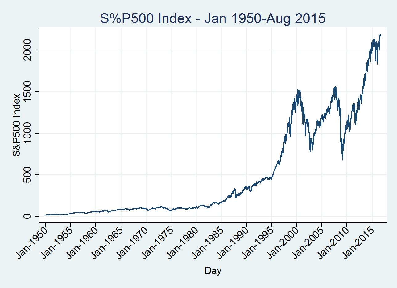
From 1950 to around 1985 the index had little variability (volatility) and it has a linear growing tendency with a small growth rate. After 1985 the rate of growth significantly increased until right before 2000. After 2000 there is a lot of volatility and recession periods since the index was decreasing for long periods of time in the years 2000-2004 and 2008-2010. In addition, this series has different average values in different periods of time, and also it has different levels of volatility for different periods.
It is possible to identify different patterns for a time-series variable and it is possible to provide personal interpretation of this pattern. The visualization of time-series variables and initial intuitive interpretation are very important before doing a more quantitative analysis using time-series models.
According to patterns related to the mean and variance of the series, and covariances among the series and its own lag values, any time-series variable can be classified in a) stationary and b) non-stationary series. Before learning more about time-series models, it is important to understand what a stationary and non-stationary series are about.
15.2 Stationary vs non-stationary series
A weakly stationary series Y_{t} has the following characteristics:
• The expected value of the series, its mean (\mu), is constant over time. In other words, no matter which periods you focus on, the average value of the series is around the same: E(Y_t)=E(Y_{t-h})=\mu for any time t and time lag h
• The variance and standard deviation of the series is around the same over time. In other words, the variance of the series is expected to be homogeneous for any period of time. Var(Y_{t})=Var(Y_{t-h})=\sigma_y^{2}
• The covariance \gamma(h) and correlation \rho(h) between one value of the series at t and its own value at a previous period t-h is the same for any time period. In other words, the covariance only depends on the time lag h.
COV(Y_{t},Y_{t-h})=COV(Y_{t},Y_{t+h})
\gamma(h)=CORR(Y_{t},Y_{t-h})=CORR(Y_{t},Y_{t+h})=\rho(h)
The concept of covariance and correlation are used to understand the relationship between two different variables. In this case we have only one variable. However, we can think that the lag of the variable (in this case, the lag h) is like another variable, so we can analyze how current values of the variable are related with its own past or future values. Actually, this type of covariance is called autocovariance, and this correlation is called autocorrelation of the time-series variable Y_{t}. It is also interesting to see that the autocovariance, autocorrelation and variance of Y_{t} are related with each other.1
The relationship is the following:
\gamma(h)=\rho(h)\sigma^{2}_{y}
A series is strictly stationary when the series satisfies the conditions for the weakly stationary series, and also satisfies other conditions related to other statistical moments of the the series: same skewness and kurtosis, and quantiles for any period of time. Since it is almost impossible to find a strictly stationary series in the real world, a weakly series is consider stationary.
Related to the S&P500 variable, we can easily see that the series is NOT stationary since its mean, variance and autocorrelations significantly increase over time. For this series it is easy to conclude that the series is not stationary. However, there are many time series variables that we cannot provide a reliable judge about stationary. In these cases, there are specific statistic tests to examine whether there is statistical evidence for stationary of a series. One of the first statistic tests for stationary is the modified Dicky-Fuller test, which will be covered later.
An interesting question would be: why is it important to know whether a series is stationary or not? The reason is that it is very difficult - if not, impossible- to model non-stationary time series, specifically series with different mean over time with no trend or pattern. A non-stationary time series can have so different behavior and patterns over time, that it will become extremely difficult to find a mathematical stochastic model to try to fit the data. However, a stationary time series is much more easy to model with a mathematical stochastic model since the expected mean and expected volatility over time are quite known.
Non-stationary series in Finance are very common, like the S&P500 index. This does not mean that we cannot model non-stationary series. Fortunately, there is a mathematical trick to transform a non-stationary series into a stationary. This trick is to apply the first or second difference to the series, or the first or second difference to the log of the series. Applying the first difference of the series is just to create another series that has the difference between the current value of Y_{t} and its previous value Y_{t-1}. The first difference of the series can be expressed as:
\triangle^{1}Y_{t}=Y_{t}-Y_{t-1}
In this case, Y_{t-1} is the first lag of the series. We can use the notation L^{1}(Y_{t}) for the first difference of the series. Then, the first difference can be expressed as:
\triangle^{1}Y_{t}=Y_{t}-L^{1}(Y_{t}) Most of the financial and economic time series variables become stationary after applying the first difference. In case that the first difference is still non-stationary, we can apply the second difference of the series, which is the first difference of the first difference. The second difference is expressed as:
\triangle^{2}Y_{t}=\triangle^{1}Y_{t}-\triangle^{1}Y_{t-1}=(Y_{t}-L^{1}(Y_{t}))-(L^{1}(Y_{t})-L^{2}(Y_{t})) \triangle^{2}Y_{t}=Y_{t}-2L^{1}(Y_{t})+L^{2}(Y_{t})=Y_{t}-2Y_{t-1}+Y_{t-2} For financial and economic series it is strongly recommended to apply natural logarithm to the variables before applying first or second differences. The reason for doing this is that the first difference of a log variable is actually the percentage increase (in continuously compounded) of the series. Another reason is that the logarithm transformation makes a non-normal variable to appear more normal, so the log of a variable has better statistical properties to be modeled. Finally, another reason is that the probability distribution of continuously compounded rates (the first log difference) is usually closer to a normal distribution compared with the distribution of the first difference.
The following graph shows the first log difference of the S&P500:
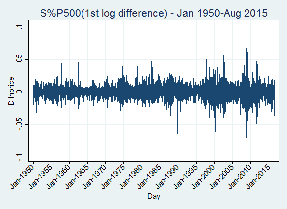
The first log difference of the index is actually the continuously compounded daily return of the index. We can see that the series has the same expected value over time. Regarding to the variance, we can see that the variance is constant for most of the time periods, except for some periods that show high volatility. If we want to model the expected value of the series (not the volatility of the series), we can use the first log difference transformation. However, we can try the second difference of the series:
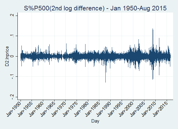 The second difference also has the same expected value over time. We can see the same level of volatility for most of the periods, except for a few periods around 1988, 2000 and 2009. Compared with the first difference graph, this one looks to have less heterogeneity of variance.
15.3 Interesting facts about time series in finance
In Finance, most of the time series variables do not satisfy the stationary condition for the homogeneity of variance. When the economy is not in crisis or recession, we can say or assume that the volatility of returns of the market stays around certain level. However, for recession or crisis periods, volatility usually increases significantly, and the volatility appears in clusters. The first mathematical models invented to fit time series data were the autoregressive moving average models (ARMA). These models assume that the series are stationary. However, in reality, there is some tolerance for the homogeneity of variance condition. A series might not look to be homogeneous in variance, but there are some statistical tests (such as the modified Dicky-Fuller test) with certain level of error that helps us to determine which variable can be considered stationary. For example, for the first log difference of the S&P500, the Dicky-Fuller test support the conclusion for stationary, even though it looks that there are certain periods with high volatility.
The first time-series autoregressive model was initially developed by Peter Whittle in 1951 2
Based on Whittle findings, George E. P. Box and Gwilym Jenkins further developed these models and published a book about ARMA models in 1976 3
Since most of the finance variables show heterogeneity of variance, in the 1980s, Robert Engle proposed and developed the Autoregressive Conditional Heteroscedasticity (ARCH) models 4
In 2003 he got the Nobel Prize in Economics mainly for his developments of the ARCH models, which significantly contributed to the Economics and Finance discipline to better understand volatility.
Once we know what a stationary time series is and why we need to assume stationary process for stochastic time series models, then I will explain the first basic time series model: the autoregressive model with 1 lag, AR(1).
15.4 Autoregressive stationary model with 1 lag, the stationary AR(1)
An AR(1) stationary model for a time series Y is defined as:
Y_{t}=\phi_{0}+\phi_{1}Y_{t-1}+\varepsilon_{t}
Where
\phi_{0},\phi_{1} are constants, and \phi_{1}<\mid1\mid
\varepsilon_{t} follows a normal distribution with mean zero 5
and constant variance \sigma^{2}_{\varepsilon}.
This models indicates that the value of Y today depends on its previous value, a specific constant and a random shock that follows a white noise process. The absolute value of the constant \phi_{1} must be less than 1 for the series to be stationary. If \mid\phi_{1}\mid>=1 then the expected value and the variance of the series are undefined, so the random series will not have any defined pattern over time and it will be totally unpredictable.
We can use basic probability theory to estimate the expected value and variance of the AR(1) stationary series. The expected value of Y_{t} will be:
E\left[Y_{t}\right]=E\left[\phi_{0}+\phi_{1}Y_{t-1}+\varepsilon_{t}\right]
Since E\left[\varepsilon_{t}\right]=0, and E\left[Y_{t}\right]=E\left[Y_{t-1}\right] because the series is assumed to be stationary, then: E\left[Y_{t}\right]=\phi_{0}+\phi_{1}E\left[Y_{t}\right] Then we can simplify the expression as:
E\left[Y_{t}\right]-\phi_{1}E\left[Y_{t}\right]=\phi_{0}
E\left[Y_{t}\right](1-\phi_{1})=\phi_{0} E\left[Y_{t}\right]=\frac{\phi_{0}}{(1-\phi_{1})}=\mu_{y}
Then the mean value of Y_{t} will converge to the value \frac{\phi_{0}}{(1-\phi_{1})} over time.
Now we can calculate the expected variance of the series:
Var(Y_{t})=Var(\phi_{0}+\phi_{1}Y_{t-1}+\varepsilon_{t})
Var(Y_{t})=Var(\phi_{0})+Var(\phi_{1}Y_{t-1})+Var(\varepsilon_{t})
Since \phi_{0} and \phi_{1} are constants and Var(\varepsilon_{t})=\sigma^{2}_{\varepsilon} then:
Var(Y_{t})=\phi^{2}_{1}Var(Y_{t-1})+\sigma^{2}_{\varepsilon}
Since the series is supposed to be stationary, then Var(Y_{t})=Var(Y_{t-1}):
Var(Y_{t})-\phi^{2}_{1}Var(Y_{t})=\sigma^{2}_{\varepsilon}
Var(Y_{t})(1-\phi^{2}_{1})=\sigma^{2}_{\varepsilon}
Var(Y_{t})=\frac{\sigma^{2}_{\varepsilon}}{(1-\phi^{2}_{1})}=\sigma^{2}_{y}
Then, on average the variance of Y_{t} will be around \frac{\sigma^{2}_{\varepsilon}}{(1-\phi^{2}_{1})} for all time periods.
If we create a random stationary series Y following the AR(1) process with specific parameters \phi_{0} and \phi_{1} in a computer program, we can check that the actual empirical mean will be very close to the theoretical mean \mu_{y}, that is \frac{\phi_{0}}{(1-\phi_{1})}, and the empirical variance of Y will be very close to the theoretical variance \sigma^{2}_{y} , which is \frac{\sigma^{2}_{\varepsilon}}{(1-\phi^{2}_{1})}.
In an AR(1) model, the \phi_{1} coefficient is actually the autocorrelation between Y_{t} and Y_{t-1}. In other words, the \phi_{1}=\rho(1). Then \phi_{1} plays the role as a filter of information between Y_{t-1} and Y_{t}. If \phi_{1}=0.7, this means that 70% of the information at Y_{t-1} is passed to Y_{t}. If we continue the process from Y_{t} to Y_{t+1}, then same filter applies, so 70% of the present value of Y will be passed to the future value Y_{t+1}. Then, we can see that the amount of information passed from Y_{t-1} to Y_{t+1} is actually 0.49 or 49%, since 0.7*0.7=0.49.
Then, the pattern we can see is that the amount of information between Y_{t-h} and Y_{t} is actually \phi^{h}_{1}. For example, the amount of information passed from 7 days ago, Y_{t-7}, to today, Y_{t}, will be 0.70^{7}=0.0823 or 8.23\%. We can see that Y_{t} will influence all future values of Y and the effect of Y_{t} on these future Y values will decay over time very quickly in an exponential way. Then, the effect of a current value of Y will have an impact to all future values. These type of stochastic processes are called processes with long-memory since the information of the time series variable will affect all future values even though this effect becomes negligible after a few periods. We can see this intuition mathematically if we analyze the AR(1) process in more detail:
Y_{t}=\phi_{0}+\phi_{1}Y_{t-1}+\varepsilon_{t}
Applying the same process to Y_{t-1} :
Y_{t-1}=\phi_{0}+\phi_{1}Y_{t-2}+\varepsilon_{t-1}
Now plugging Y_{t-1} equation in the first equation:
Y_{t}=\phi_{0}+\phi_{1}(\phi_{0}+\phi_{1}Y_{t-2}+\varepsilon_{t-1})+\varepsilon_{t}
Y_t=\phi_{0}(1+\phi_{1})+\phi^{2}_{1}Y_{t-2}+\phi_{1}\varepsilon_{t-1}+\varepsilon_{t} We can continue the process by plugging the formula for Y_{t-2}:
Y_{t}=\phi_{0}(1+\phi_{1})+\phi^{2}_{1}(\phi_{0}+\phi_{1}Y_{t-3}+\varepsilon_{t-2})+\phi_{1}\varepsilon_{t-1}+\varepsilon_{t} Y_{t}=\phi_{0}(1+\phi_{1}+\phi^{2}_{1})+\phi^{3}_{1}Y_{t-3}+\phi^{2}_{1}\varepsilon_{t-2}+\phi_{1}\varepsilon_{t-1}+\varepsilon_{t} If we continue the plugging for all possible lag values of Y, then we will arrive to something like:
Y_{t}=\phi_{0}(1+\phi_{1}+\phi^{2}_{1}+...+\phi^{\infty}_{1})+\phi^{\infty}_{1}Y_{t-\infty}+(\varepsilon_{t}+\phi_{1}\varepsilon_{t-1}+\phi^{2}_{1}\varepsilon_{t-2}+\phi^{3}_{1}\varepsilon_{t-3}+...+\phi^{\infty}_{1}\varepsilon_{t-\infty})
Since \mid\phi_{1}\mid<1, then \phi^{\infty}_{1}=0, and the mathematical series (1+\phi_{1}+\phi^{2}_{1}+...+\phi^{\infty}_{1}) converges to \frac{1}{(1-\phi_{1})} according to a Taylor expansion, then:
Y_{t}=\frac{\phi_{0}}{(1-\phi_{1})}+(\varepsilon_{t}+\phi_{1}\varepsilon_{t-1}+\phi^{2}_{1}\varepsilon_{t-2}+\phi^{3}_{1}\varepsilon_{t-3}+...+\phi^{\infty}_{1}\varepsilon_{t-\infty}) Then: Y_{t}=\frac{\phi_{0}}{(1-\phi_{1})}+\sum^{\infty}_{h=0}(\phi^{h}_{1}\varepsilon_{t-h})=\mu_{y}+\sum^{\infty}_{h=0}(\phi^{h}_{1}\varepsilon_{t-h}) Since \mu_{y}=\frac{\phi_{0}}{(1-\phi_{1})} then:
Y_{t}=\mu_{y}+\sum^{\infty}_{h=0}(\phi^{h}_{1}\varepsilon_{t-h})
Then, this is another mathematical way to express the AR(1) model, as an infinite sum of errors or random shocks. In this model we can see the long-term memory of the process since the value of Y today depends on all previous random shocks. Actually, the value of Y_{t} will be equal to its mean plus a weighted average of all previous errors or random shocks. The more recent shocks have much more weight than the old shocks (for old shocks, h is large, so the weight \phi^{h}_{1} is almost zero). It is said that the AR(1) process can be expressed as a Moving Average model with infinite terms (MA(q) when q tends to infinite). We will review the MA(q) models in the following note.
If we take the expected value of this expression, we will get \frac{\phi_{0}}{(1-\phi_{1})} since the expected value of the errors is zero.
In autoregressive models, the term random error \varepsilon_{t} is also called a random shock at time t. In the example of the S&P continuously compounded returns, that is the first log difference of the index, we can model this series as an AR(1) model. In this case, we can say that the expected return of the S&P tomorrow will be equal to the return of today multiplied by the filter \phi_{1} plus a constant \phi_{0} plus a random shock. This random shock is supposed to be the effect of all news of tomorrow that will affect the index return. Since we are modeling the market index of 500 firms, then all the news for all 500 firms will be summarized in this random shock \varepsilon_{t+1}.Then following the previous mathematical expression, the return of the market index S&P500 today is equal to its overall mean plus all random daily shocks since the first day of the index (in 1957 the index started with 500 firms).
We can generalize an autoregressive process to AR(p), where we include not only 1 lag, but p lags in the model.
16 The Random Walk Model
If the coefficient \mid\phi_{1}\mid>=1, then the AR(1) process becomes non-stationary since its variance and its expected value are not constant, and are usually growing with time. Assuming that this series is stationary, its mean or expected value is \frac{\phi_{0}}{(1-\phi_{1})}. When \phi_{1} is very close to 1, then the expected value will be a very big number. A similar thing happens with the expected variance \frac{\sigma^{2}_{\varepsilon}}{(1-\phi^{2}_{1})}. If \phi_{1} is very close to 1, then the variance becomes very big, meaning that the expected volatility is too big and impossible to determine over time.
If the coefficient \mid\phi_{1}\mid=1, then the AR(1) process is called a random walk. Then, a random walk can be expressed as:
Y_{t}=\phi_{0}+Y_{t-1}+\varepsilon_{t}
We can also express the same process in a similar way we did with the stationary AR(1) process:
Y_{t}=\phi_{0}+(\phi_{0}+Y_{t-2}+\varepsilon_{t-1})+\varepsilon_{t}=2\phi_{0}+Y_{t-2}+\varepsilon_{t-1}+\varepsilon_{t} Y_{t}=2\phi_{0}+(\phi_{0}+Y_{t-3}+\varepsilon_{t-2})+\varepsilon_{t-1}+\varepsilon_{t}=3\phi_{0}+Y_{t-3}+\varepsilon_{t-2}+\varepsilon_{t-1}+\varepsilon_{t} After doing this substitution repeatedly until the initial Y, and assuming that the initial value of Y is {o}, then we can express Y{t} as
Y_{t}=t\phi_{0}+\varepsilon_{1}+\varepsilon_{2}+...+\varepsilon_{t}
Since the expected value of the errors is zero, then the expected value the this random walk will be:
E\left[Y_{t}\right]=t\phi_{0}+E\left[\varepsilon_{1}+\varepsilon_{2}+...+\varepsilon_{t}\right]=t\phi_{0}
We can see that the expected value (mean) of Y will depend on t and \phi_{0}. If \phi_{0} is zero, then the expected value of the random walk will be zero. If \phi_{0} is not zero, then the expected value will not be constant and will depend on t.
The expected variance of a random walk can be estimated as follows:
Var(Y_{t})=Var(\varepsilon_{1}+\varepsilon_{2}+...+\varepsilon_{t})=Var(\varepsilon_{1})+Var(\varepsilon_{2})+...+Var(\varepsilon_{t})=t\sigma^{2}_{\varepsilon}
The expected variance will be linearly increasing with time, so the variance will not be constant.
Then we can see that the random walk process is not mean-reverting as in the case of the AR(1) stationary series.
If the coefficient \mid\phi_{1}\mid>1, the AR(1) process becomes explosive in the sense that it does not have an expected value, and its variance will increase exponentially over time.
When the lag h is zero, then the covariance actually becomes the variance of the series: COV(Y_{t},Y_{t-0})=\gamma(0)=Var(Y_{t})=\sigma_y^{2} We can also see how the autocovariance and autocorrelation are related. From basics statistics we know that correlation is the standardized version of the covariance between two variables. In the context of time-series variables, the autocorrelation is the standardized version of the autocovariance of the variable considering a specific lag of the variable. the In other words, the autocorrelation is equal to the autocovariance divided by the product of standard deviations of the variable, that is the same in the case of a time-series variable. In this case, the autocorrelation is:\rho(h)=\frac{\gamma(h)}{\sqrt{\sigma^{2}_{y}}\sqrt{\sigma^{2}_{y}}}=\frac{\gamma(h)}{\sigma^{2}_{y}}=\frac{\gamma(h)}{\gamma(0)}. Then the autocovariance is equal to the autocorrelation times the variance of the variable: \gamma(h)=\rho(h)\sigma_y^{2}.↩︎
In his thesis “Hypothesis testing in time series analysis” in 1951, Peter Whittle describes the foundations of an ARMA model↩︎
Box, G.E.P. and Jenkins, G.M. (1976), “Time series analysis: forecasting and control”, revised ed., Holdden-Day, San Francisco, CA↩︎
Engle, Robert F. (1982), “Autoregressive Conditional Heteroscedasticity with Estimates of the Variance of United Kingdom Inflation, Econometrica, 50(4), pp. 987-1008. In this paper Robert Engle developed the foundations of the ARCH models.↩︎
This is usually called a Gaussian (normal) white noise random variable that follows an identically and independent normally distributed process (i.i.d.)↩︎