7 Chapter 7 - Hypothesis Testing

The idea of hypothesis testing is to provide strong evidence - using facts - about a specific belief that is usually supported by a theory or common sense. This belief is usually the belief of the person conducting the hypothesis testing. This belief is called the Alternative Hypothesis.

The person who wants to show evidence about his/her belief is supposed to be very humble so the only way to be convincing is by using data and a rigorous statistical method.

Let’s imagine 2 individuals, Juanito and Diablito. Juanito wants to convince Diablito about a belief. Diablito is very, very skeptical and intolerant. Diablito is also an expert in Mathematics and Statistics! Then, Juanito needs a very robust statistical method to convince and persuade Diablito. Juanito also needs be very humble so Diablito does not get angry.

Then, Juanito decides to start assuming that his belief is NOT TRUE, so Diablito will be receptive to continue listening Juanito. Juanito decides to collect real data about his belief and decide to define 2 hypotheses:

H0: The Null Hypothesis. This hypothesis states the opposite of Juanito’s belief, but he starts accepting that this hypothesis is TRUE.
Ha: The Alternative Hypothesis. This is what Juanito beliefs, but he starts accepting that this is NOT TRUE.

Diablito is an expert in Statistics, so he knows the Central Limit Theorem very well! However, Juanito is humble, but he also knows the CLT very well.

Then Juanito does the following to try to convince Diablito:

Juanito collects a random sample related to his belief. Imagine that his belief is about the mean of a variable X; he believes that the mean of X is greater than zero.
He calculates the mean and standard deviation of the sample.

Since he collected a random sample, then he and Diablito know that, thanks to the CLT:

The mean of this sample will behave VERY SIMILAR to a normal distribution,
The standard deviation of this sample mean is much less than the standard deviation of the individuals of the sample and this can be calculated by dividing the individual standard deviation by the square root of sample size.

Since this sample mean will behave like a normal distributed variable, then there is a probability of about 95% that the real mean will in the range: [Sample Mean - 2 Standard Deviation .. Sample Mean + 2 Standard Deviations].

Then, if Juanito shows that the calculated sample mean of X is equal or higher than zero plus 2 standard deviations, then Juanito will have a very powerful statistical evidence to show Diablito that the probability that the true mean of X is bigger than zero. In other words, Juanito can say that the probability that the true mean of X is greater than zero is about 95%.

Juanito is very smart (as Diablito). Then, Juanito calculates an easy measure to quickly know how far its sample mean is away from the hypothetical mean (zero), but measured in # of standard deviations of the mean. This new standardized distance is usually called z or t. If |z| is 2 or more, the he has strong evidence to say that the sample mean is 2 standard deviations above the supposed true mean (zero), so he could convince Diablito about his belief that the actual TRUE mean is greater than zero.

Although the CLT says that the mean of a sample behaves as normal, it has been found that the CLT is more consistent with the t-Student probability distribution. Actually, the t-Student distribution is very, very similar (almost the same) to the normal distribution when the sample size is bigger than 30. But for small samples, the t-Student does a much better job in representing what happens with the CLT for small samples compared with the z normal distribution.

Then, for hypothesis testing we will use the t-Student distribution instead of the z normal distribution.

The hypothesis testing to compare the mean of a variable with a value or with another mean is called one-sample t-test.

We can use the same method of hypothesis testing for other types of random variables. For example, hypothesis testing is automatically performed to model coefficients when we run any linear regression model, which is very popular in machine learning.

For now, I will illustrate the method of hypothesis testing for the simple case of testing whether the mean of a variable is different to a specific value - the one-sample t-test.

7.1 One-sample t-test

Imagine that I believe that investing in the S&P 500 index is a good long-term investment. The S&P500 index is a portfolio composed of the largest 500 US public firms. If I believe this, at least I have to show statistical evidence that the mean of monthly return of the S&500 is greater than zero, so when I compound this monthly return to long periods, the long-term investment will be positive and attractive.

The steps for doing a hypothesis test are the following:

Identify the variable of study for the hypothesis test. In this case, it can be the monthly average return of the S&P500: \bar{X}.
State the null and the alternative hypothesis using the variable of study. The alternative hypothesis is my believe, and the null hypothesis is the opposite to my believe. I start considering that the Null Hypothesis is 100% TRUE, and my alternative hypothesis is completely FALSE. Then, the purpose of the test is to find evidence to REJECT the Null Hypothesis.

We have to distinguish between the sample variable and the population variable. In this case, the sample variable is the sample mean that I will calculate after collecting historical monthly returns of the S&P500. The population mean will be the TRUE variable of the population, which in this case can be considered as the whole future of the monthly returns of the S&P500. Then:

\mu = Population Mean

\bar{X} = Sample Mean

In this example, the hypothesis can be stated as:

H0 (Null hypothesis): \mu=0 (Initially considered as 100% TRUE)

Ha (Alternative hypothesis): \mu>0 (Initially considered as FALSE)

Collect data that measures the variable of study. It is recommended collecting a representative sample from the population of the variable. In the case of cross-sectional variables, it is recommended to pick a representative random sample. For time-series variables - such as the historical monthly returns of the S&P500- we need to make some assumptions.

In this example, the variable of study is actually a time-series variable, so the individuals that can be collected are actually historical monthly returns. Here I need to do an assumption that my horizon for my investment is about 3 years, and I assume that the average return of the S&P500 will remain very similar than the average monthly return for the last 3-years. This is a very straight-forward assumption, that many people would not agree, but for the sake of this example, I will accept my assumption.

Calculate the t-Statistic of the test. The t-Statistic is a measure of how far away the sample variable - in this case, the sample mean - is away from the hypothetical value of the population variable - in this case, it is zero (the value of variable stated in the Null hypothesis). We can call the t-Statistic as a standardized distance of the sample variable from its hypothetical true value. This standardized distance is measured in # of Standard Deviations of the variable of study - in this case, the sample mean of the S%P monthly returns.

Then, I can define the t-Statistic as the following:

t-Statistic=\frac{\bar{X}-0}{\sigma_{\bar{X}}} Where \sigma_{\bar{X}} is the Standard Deviation of the Variable of Study, which in this case, it is the monthly average return of the S&P500.

The numerator of this formula is the raw distance of the sample variable from the hypothetical value, which in this case it is zero. When we devide this distance by its standard deviations, then the measure of this distance will be in # of standard deviations.

In Statistics, the Standard Deviation of the Variable of Study is called Standard Error.

Then, I need to calculate both, 1) the sample variable, which in this case is the sample mean of historical monthly returns of the S&P, and 2) The sample standard error, which in this caes is the standard deviation of the sample mean of monthly returns of the S&P500.

Calculate the p-value of the test, which is the probability that I will be wrong if I reject this Null Hypothesis - giving support for my hypothesis, which is the alternative hypothesis.

Since the p-value is the probability of making a mistake rejecting the null hypothesis, then we can say that the confindence level of the test is the reciprocal of the pvalue. In other words, there is a probability of (1-pvalue) that my conclusion of rejecting the null is true!

How can I calculate the p-value?

Make the conclusion of the test:

If the p-value is less or equal to 0.05 (5%), then I can say that with a 95% confidence, I can reject the NULL Hypothesis, and provide strong evidence to my hypothesis.
If the p-value is greater than 0.05 (5%), then I do not have evidence at the 95% confidence level to reject the Null hypothesis, so I cannot provide strong support for my hypothesis.

In reality, we have to apply our judgement to make the final conclusion! We can play with different levels of confidence, not only at the 95% level. How can I do this?

Note: we can also use the t-Statistic to make a conclusion instead of the p-value. There is a straight-forward relationship for the values of t-Statistic and p-values, according to the sample size (number of observations of the random sample).

A general rule-of-thumb is that if |t|>=2, then the pvalue<0.05, so I could reject the null hypothesis if the absolute value of t-Statistic is greater or equal to 2.

7.2 Example of on-sample t-test

Imagine that you believe that investing in the US financial market is a good long-term investment. You have been learning about the financial performance of the largest US companies for the last 3 years, and also the leadership of US tech firms -such as Microsoft, Google, Meta, Nvidia- in the Artificial Intelligence innovations and applications.

Step 1 - Identify the variable of study

In the world of investment, there is a quick way to invest in the whole US market if you just buy a market index. In this case, you can buy the S&P500 index, which is a virtual portfolio composed of the largest 500 US companies. Then, you define that the variable of study will be the average monthly return of the S&P500 index

Step 2 - State the hypotheses

Then, you decide first to show that the average monthly return of the S&P500 is positive. After showing this, you plan to do a comparative analysis with other alternative investments. But for now, you just want to show that the average monthly return of the S&P is positive. Then, you decide to run a one-sample t-test to convice your father, who told you he will support you if you save your money in a good long-term investment.

Then, the stated hypotheses are:

In this example, the hypothesis can be stated as:

H0 (Null hypothesis): \mu=0 (Initially considered as 100% TRUE)

Ha (Alternative hypothesis): \mu>0 (Initially considered as FALSE)

Where:

\mu = Population Mean, which in this case is the overall monthly average return of the S&P500 index

\bar{X} = Sample Mean, which in this case is the actual monthly average return of the S&P500 index for the last 3 years

Step 3 - Collect data to measure the variable of study.

In this case, we can collect real data of past monthly quotations (like prices) for the S&P500 from Yahoo-Finance:

We download historical monthly data for the S&P500 market index. In this case, the variable of study is the average monthly return, so I need do a transformation from monthly quotations (prices) to monthly returns.

In most Statistical analysis, when dealing with percentages, it is very recommended to use logaritmic percentage changes, which in this context is called continuously compounded (cc) returns.

Here is the code to collect the S&500 monthly quotations and transforming them to cc returns:

import yfinance as yf
import numpy as np
import pandas as pd
import matplotlib
import matplotlib.pyplot as plt

# Download stock data
data = yf.download('^GSPC', start='2020-01-01', end='2025-07-31', interval='1mo', auto_adjust=True)
adjprices = data['Close']  # Get adjusted close prices

# Calculate continuously compounded returns as the difference of the log prices:

ccr = np.log(adjprices) - np.log(adjprices.shift(1))
ccr = ccr.dropna()

Step 4 - Calculate the t-Statistic of the test.

# H0: mean(ccr$GSPC) = 0
# Ha: mean(ccr$GSPC) <> 0

# Standard error
se_GSPC = np.std(ccr,ddof=1) / np.sqrt(len(ccr))
print(f"Standard error S&P 500 = {se_GSPC}")

# t-value
mean_ccr = np.mean(ccr)
t_GSPC = (mean_ccr - 0) / se_GSPC
print(f"t-value S&P 500 = {t_GSPC}")

Standard error S&P 500 = Ticker
^GSPC    0.00635
dtype: float64
t-value S&P 500 = Ticker
^GSPC    1.612253
dtype: float64

C:\Users\L00352955\AppData\Roaming\Python\Python313\site-packages\numpy\_core\fromnumeric.py:4062: FutureWarning:

The behavior of DataFrame.std with axis=None is deprecated, in a future version this will reduce over both axes and return a scalar. To retain the old behavior, pass axis=0 (or do not pass axis)

Using the t-Statistic we can start doing a preliminar conclusion before calculating the corresponding p-value of the test. Since the t-value of the mean return of S&P 500 is lower than 2, I can’t reject the null hypothesis at the 95% confidence level. Therefore, at the 95% confidence level, S&P 500 mean return is not statistically greater than 0. However, we have to apply our judgement to make the final conclusion!

Step 5 - Calculate the p-value of the test

We can calculate the p-value of the test.

Reminding what is the p-value of a test:

The p-value of a test is the probability that I will be wrong if I reject the NULL hypothesis. In other words, (1-pvalue) will be the probability that MY HYPOTHESIS (the alternative hypothesis) is true!

(1-pvalue)% is called the confidence level I can use to reject the null hypothesis.

We can calculate any p-value with the following parameters:

t-Statistic
Degrees of freedom, which in this case is equal to the number of sample observations minus 1

Then, there is a direct relationship between t-Statistic and p-value.

Unfortunately, there is no quick formula to calculate the p-value of a test. Why? because the p-value is a probability, and it can be found calculating the integral of the probability density function, in this case, the t-Student probability function. The only way to calculate this integral is throuth a numerical algorithm (programming loop that optimizes the solution for the area under the curve).

Fortunately, most computer software and programming languages such as Excel, Python, etc. can easily calculate this p-value given a t-Statistic and the number of observations. Below I illustrate how to calculate the pvalue in Python:

from scipy import stats as st

# One-sided t-test
ttest_GSPC = st.ttest_1samp(ccr, 0, alternative='greater')

# Showing the t-Statistics and the p-value:
ttest_GSPC

TtestResult(statistic=array([1.61225307]), pvalue=array([0.05587612]), df=array([65]))

Actually this function automatically calculates the t-Statistic and the p-value.

See that I got the same value for the t-Statistic than the value I calculated above.

The p-value that is calculated here is the 1-tailed p-value since I specified the parameter alternative = ‘greater’.

Actually there are 2 types of p-values:

1-tailed p-value
2-tailed p-value

What are these p-values? In this example, since my belief is that the monthly return will be positive (1-tailed), then I can use the 1-tailed p-value. The 2-tailed p-value is always equal to the double of the 1-tailed p-value, so it is a more conservative p-value. When we use the 2-tailed p-value? we can use the 2-tailed p-value when our belief is not quite clear, but we believe that the value of the variable is DIFFERENT to a specific value. We can also use 2-tailed p-value to be more conservative with our analysis. In this case, I will keep using the 1-tailed p-value.

Step 6 - Make a conclusion for the test

The p-value was py$ttest_GSPC.value[0], so it is just a little bit greater than 5%. Then, in a strict way, I cannot say that I have evidence at the 95% confidence level to reject the null. Does this mean that investing in the S&P is not going to give you positive returns over time? No, this is not quite a good conclusion.

We can calculate the confidence level of the test, which is equal to (1-pvalue):

confidence_level = 1 - ttest_GSPC.pvalue[0] 

print(f"The confidence level is = {confidence_level}")

The confidence level is = 0.9441238817541077

Then, I can say that I reject the null hypothesis (that the monthly average of the S&P is equal to zero) at the 100*py$confidence_level% confidence level, which still can be considered as strong statistical evidence.

In other words, we can accept our hypothesis that monthly mean return of the S&P500 is >0 at the py$confidence_level % (=1-pvalue)!

In Statistics, when the p-value of the test is less or equal to 0.05 we can say that our result is statistically significant. When the p-value is between 0.05 and 0.10 we can say that our results were marginally significant.

I will illustrate another type of hypothesis test, which is called 2-sample t-test. I will illustrate this with a practical example.

7.3 Hypothesis testing - two-sample t-test

Now we will do a hypothesis testing to compare the means of two groups. This test is usually named two-sample t-test.

In the case of the two-sample t-test we try to check whether the mean of a group is greater than the mean of another group.

Imagine we have two random variables X and Y and we take a random sample of each variable to check whether the mean of X is greater than the mean of Y.

We start writing the null and alternative hypothesis as follows:

H0:\mu_{x}=\mu_{y}

Ha:\mu_{x}\neq\mu_{y}

We do simple algebra to leave a number in the right-hand side of the equality, and a random variable in the left-hand side of the equation. Then, we re-write these hypotheses as:

H0:(\mu_{x}-\mu_{y})=0

Ha:(\mu_{x}-\mu_{y})\neq0

The Greek letter \mu is used to represent the population mean of a variable.

To test this hypothesis we take a random sample of X and Y and calculate their means.

Then, in this case, the variable of study is the difference of 2 means! Then, we can name the variable of study as diff:

diff = (\mu_{x}-\mu_{y})

Since we use sample means instead of population means, we can re-define this difference as:

diff = (\bar{X}-\bar{Y})

The steps for all hypothesis tests are basically the same. What changes is the calculation of the standard deviation of the variable of study, which is usually names standard error.

For the case of one-sample t-test, the standard error was calculated as \frac{SD}{\sqrt{N}}, where SD is the individual sample standard deviation of the variable, and N is the sample size.

In the case of two-sample t-test, the standard error SE can be calculated using different formulas depending on the assumptions of the test. In this workshop, we will assume that the population variances of both groups are NOT EQUAL, and the sample size of both groups is the same (N). For these assumptions, the formula is the following:

SD(diff)=SE=\sqrt{\frac{Var(X)+Var(Y)}{N}}

But, where does this formula come from?

We can easily derive this formula by applying basic probability rules to the variance of a difference of 2 means. Let’s do so.

The variances of each group of X and Y might be different, so we can estimate the variance of the DIFFERENCE as:

Var(\bar{X}-\bar{Y})=Var(\bar{X})+Var(\bar{Y})

This is true if only if \bar{X} and \bar{Y} are independent. We will assume that both random variables are not dependent of each other. This might not apply for certain real-world problems, but we will assume that for simplicity. If there is dependence I need to add another term that is equal to 2 times the covariance between both variables.

Why the variance of a difference of 2 random variables is the SUM of their variance? This sounds counter-intuitive, but it is correct. The intuition behind this is that when we make the difference we do not know which random variable will be negative or positive. If a value of \bar{Y}_i<0 then we will end up with a SUM instead of a difference!

As we learned in the CLT, the variance of the mean of a random variable is reduced according to its sample size: Var(\bar{X)}=\frac{Var(X)}{N}. Then:

Var(\bar{X}-\bar{Y})=\frac{Var(X)}{N}+\frac{Var(Y)}{N}

Factorizing the expression:

Var(\bar{X})=\frac{1}{N}\left[Var(X)+Var(Y)\right]

We take the squared root to get the expected standard deviation of (\bar{X}-\bar{Y}):

SD(\bar{X})=\sqrt{\frac{1}{N}\left[Var(X)+Var(Y)\right]}

Then, the method for hypothesis testing is the same we did in the case of one-sample t-test. We just need to use this formula as the denominator of the t-statistic.

The, the t-statistic for the two-sample t-test is calculated as:

t=\frac{(\bar{X}-\bar{Y})-0}{\sqrt{\frac{Var(X)+Var(Y)}{N}}}

Remember that the value of t is the # of standard deviations of the variable of study (in this case, the difference of the 2 means) that the empirical difference we got from the data is away from the hypothetical value, zero.

The rule of thumb we have used is that if |t|>2 we have have statistical evidence at least at the 95% confidence level to reject the null hypothesis (or to support our alternative hypothesis).

7.4 EXAMPLE - IS AMD MEAN RETURN HIGHER THAN ORACLE MEAN RETURN?

Do a t-test to check whether the mean monthly cc return of AMD (AMD) is significantly greater than the mean monthly return of Intel. Use data from Jan 2020 to date_

# Getting price data. I indicate getting adjusting prices as close prices:
sprices=yf.download(tickers='AMD ORCL', start='2020-01-01', end='2025-01-31',interval='1mo', auto_adjust=True)
# I select the Close columns for both stocks:
sprices=sprices['Close']

[                       0%                       ][*********************100%***********************]  2 of 2 completed

The sprices data frame has 2 columns: close price for AMD and close price for INTC:

sprices.head(5)

Ticker	AMD	ORCL
Date
2020-01-01	47.000000	47.949932
2020-02-01	45.480000	45.417725
2020-03-01	45.480000	44.380085
2020-04-01	52.389999	48.640858
2020-05-01	53.799999	49.610043

Now we calculate monthly continuously compounded returns for both stocks:

# Calculating cc returns as the difference of the log price and the log price of the previous month:
sr = np.log(sprices) - np.log(sprices.shift(1))
# we can also calculate cc returns using the diff function:
# sr = np.log(sprices).diff(1)

# Deleting the first month with NAs:
sr=sr.dropna()

sr.head()

Ticker	AMD	ORCL
Date
2020-02-01	-0.032875	-0.054255
2020-03-01	0.000000	-0.023112
2020-04-01	0.141443	0.091673
2020-05-01	0.026558	0.019729
2020-06-01	-0.022367	0.027515

We can calculate the monthly mean return for both stocks:

amd_mean = sr['AMD'].mean()
orcl_mean = sr['ORCL'].mean()
print(f"AMD mean cc % return= {100*amd_mean}%")
print(f"Oracle mean cc % return= {100*orcl_mean}%")

AMD mean cc % return= 1.5050190594531336%
Oracle mean cc % return= 2.089094754052699%

We can see that, on average, Oracle mean return is higher than the AMD mean return. However, we need to check whether this difference is statistically significant. Then, we need to do a 2-sample t-test.

We state the hypothesis and calculate the t-Statistic:

# Stating the hypotheses: 
# H0: (mean(rAMD) - mean(rORACLE)) = 0
# Ha: (mean(rAMD) - mean(rORACLE)) <> 0

# Calculating the standard error of the difference of the means:
# Getting the number of non-missing observations for the sample:
N = sr['AMD'].count()
# Getting the variances of both columns: 
amd_var = sr['AMD'].var()
orcl_var = sr['ORCL'].var()
# Now we get the standard error for the mean difference:
sediff = np.sqrt((1/N) * (amd_var + orcl_var ) )

# Calculating the t-Statistic:
t = (sr['AMD'].mean() - sr['ORCL'].mean()) / sediff
print(f"t-Statistic = {t}")

t-Statistic = -0.2678502434577802

Fortunately we can use a Python function to easily calculate the t-value along with its p-value and 95% confidence interval:

# I do the 2-way sample t-test using the ttest_ind function from stats:
st.ttest_ind(sr['AMD'],sr['ORCL'],equal_var=False)
# With this function we avoid calculating all steps of the hypothesis test!

TtestResult(statistic=np.float64(-0.2678502434577802), pvalue=np.float64(0.7894068075259335), df=np.float64(93.15008644487645))

We got the same t-value as above, and also we got the p-value of the test. Since the t-value is much greater than 2, and pvalue is much greater than 0.05, we cannot reject the null hypothesis.

Then, although the ORCL mean return is higher than that of AMD, we do not have significance evidence (at the 95% confidence) to say that the mean of ORCL return is greater than the mean of AMD return.

We can use another Python function that display more results for this t-test:

import researchpy as rp
# Using the ttest function from researchpy:
rp.ttest(sr['AMD'],sr['ORCL'],equal_variances=False)
# With this function we avoid calculating all steps of the hypothesis test!

C:\Users\L00352955\AppData\Roaming\Python\Python313\site-packages\researchpy\ttest.py:301: FutureWarning:

Setting an item of incompatible dtype is deprecated and will raise an error in a future version of pandas. Value 'AMD' has dtype incompatible with float64, please explicitly cast to a compatible dtype first.

C:\Users\L00352955\AppData\Roaming\Python\Python313\site-packages\researchpy\ttest.py:460: FutureWarning:

Setting an item of incompatible dtype is deprecated and will raise an error in a future version of pandas. Value 'Difference (AMD - ORCL) = ' has dtype incompatible with float64, please explicitly cast to a compatible dtype first.

(   Variable      N      Mean        SD        SE  95% Conf.  Interval
 0       AMD   60.0  0.015050  0.147082  0.018988  -0.022945  0.053045
 1      ORCL   60.0  0.020891  0.083049  0.010722  -0.000563  0.042345
 2  combined  120.0  0.017971  0.118970  0.010860  -0.003534  0.039475,
          Satterthwaite t-test  results
 0  Difference (AMD - ORCL) =   -0.0058
 1       Degrees of freedom =   93.1501
 2                        t =   -0.2679
 3    Two side test p value =    0.7894
 4   Difference < 0 p value =    0.3947
 5   Difference > 0 p value =    0.6053
 6                Cohen's d =   -0.0489
 7                Hedge's g =   -0.0486
 8           Glass's delta1 =   -0.0397
 9         Point-Biserial r =   -0.0277)

If you receive an error, you might need to install the researchpy package with the command:

!pip install researchpy

We got the same results as above, but now we see details about the mean of each stock, the difference, the tvalue, and the pvalue of the difference!

7.5 Confidence level, Type I Error and p-value

The confidence level of a test is related to the error level of the test. For a confidence level of 95% there is a probability that we make a mistaken conclusion of rejecting the null hypothesis. Then, for a 95% confidence level, we can end up in a mistaken conclusion 5% of the time. This error is also called the Type I Error.

The pvalue of the test is actually the exact probability of making a Type I Error after we calculate the exact t-statistic. In other words, the pvalue is the probability that we will be wrong if we reject the null hypothesis (and support our hypothesis).

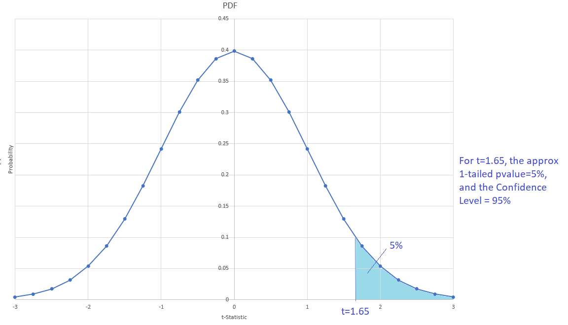
For each value of a t-statistic, there is a corresponding pvalue. We can relate both values in the following figure of the t-Student PDF:

For a 95% confidence level and 2-tailed pvalue, the critical t value is close to 2 (is not exactly 2); it can change according to N, the # of observation of the sample.

When the sample size N>30, the t-Student distribution approximates the Z normal distribution. In the above figure we can see that when N>30 and t=2, the approximates pvalues are: 1-tailed pvalue = 2.5%, and 2-tailed pvalues=5%.

Then, what is 1-tailed and 2-tailed pvalues? The 2-tailed pvalue will always be twice the value of the 1-tailed pvalue since the t-Student distribution is symmetric.

We always want to have a very small pvalue in order to reject H0. Then, the 1-tailed pvalue seems to be the one to use. However, the 2-tailed pvalue is a more conservative value (the diablito will feel ok with this value). Most of the statistical software and computer languages report 2-tailed pvalue.

Then, which pvalue is the right to use? It depends on the context. When there is a theory that supports the alternative hypothesis, we can use the 1-tailed pvalue. For now, we can be conservative and use the 2-tailed pvalue for our t-tests.

Then, we can define the p-value of a t-test (in terms of the confidence level of the test) as:

pvalue=(1-ConfidenceLevel)

In the case of 1-tailed pvalue and a 95% confidence evel, the critical t-value is less than 2; it is approximately 1.65: