Every regression model we have estimated so far came with a set of assumptions, listed in Chapter 9. Estimating the model is easy; checking whether we were entitled to is the work that separates an analyst from a button-pusher.
This chapter covers the practical diagnosis of a multiple regression model:
Multicollinearity — what it is, how to detect it, and what to do about it
Extreme values of X — leverage points
Outlier observations — points the model fits badly
Influential observations — the intersection of the two, and the ones that actually matter
Heteroskedasticity and autocorrelation — when the standard errors lie
A useful way to organize the whole chapter: some problems make your coefficients wrong, and others make your standard errors wrong. The first kind is far more serious, because no amount of additional data will fix it.
A map of what can go wrong
Problem
Coefficients biased?
Standard errors wrong?
Severity
Omitted variable
Yes
Yes
Critical
Influential outlier
Yes (in effect)
Yes
High
Multicollinearity
No
Yes (inflated)
Moderate
Heteroskedasticity
No
Yes
Moderate
Autocorrelation
No
Yes (usually understated)
Moderate
Let’s set up a small dataset to work with throughout the chapter.
import numpy as npimport pandas as pdimport matplotlib.pyplot as pltimport statsmodels.api as smimport statsmodels.formula.api as smfrng = np.random.default_rng(2026)n =120# Three firm characteristics; note that x3 is built to be nearly a copy of x2:x1 = rng.normal(50, 12, n) # firm size indexx2 = rng.normal(20, 5, n) # advertising spendx3 =2* x2 + rng.normal(0, 0.6, n) # marketing headcount (nearly collinear with x2)y =30+0.8*x1 +1.5*x2 + rng.normal(0, 6, n) # salesfirms = pd.DataFrame({"sales": y, "size": x1, "adspend": x2, "mktg_staff": x3})firms.describe().round(2)
sales
size
adspend
mktg_staff
count
120.00
120.00
120.00
120.00
mean
101.28
50.59
20.46
40.93
std
13.98
12.26
5.57
11.23
min
64.52
22.54
1.26
2.13
25%
92.91
42.03
16.61
33.57
50%
100.59
49.67
20.74
41.27
75%
110.44
58.15
23.93
48.00
max
135.59
87.81
34.59
69.20
14.1 Multicollinearity
Multicollinearity exists when two or more independent variables are highly correlated with each other. It comes in two flavours:
Perfect multicollinearity, where one variable is an exact linear combination of others. The model simply cannot be estimated — this is the dummy variable trap of Chapter 13.
Near multicollinearity, where the correlation is high but not exact. The model can be estimated, and this is the dangerous case, because nothing appears to go wrong.
14.1.1 Why it is a problem
Recall from Chapter 10 that the precision of a coefficient depends on how much independent variation its variable has. In a multiple regression, b_1 is estimated from the variation in X_1 that is not shared with the other predictors. If X_1 and X_2 move almost in lockstep, there is very little unique variation left, and the model cannot tell which of the two deserves the credit.
The consequence is a characteristic and easily recognized symptom:
Coefficients become unstable and standard errors become large, while the model as a whole fits well.
You will see a high R^2, a significant F-test, and yet individually insignificant t-statistics — sometimes with coefficients of the wrong sign. That combination is nearly diagnostic of multicollinearity.
Let’s produce it deliberately:
m_clean = smf.ols("sales ~ size + adspend", data=firms).fit()m_multi = smf.ols("sales ~ size + adspend + mktg_staff", data=firms).fit()print("--- Model WITHOUT the collinear variable ---")print(m_clean.summary().tables[1])print(f"R-squared = {m_clean.rsquared:.4f}\n")print("--- Model WITH the collinear variable ---")print(m_multi.summary().tables[1])print(f"R-squared = {m_multi.rsquared:.4f}")
Compare the two outputs. Adding mktg_staff — which carries almost no information beyond adspend — barely changes R^2, but the standard error on adspend explodes and both marketing coefficients become individually insignificant. The model has not become less accurate; it has become less able to attribute the effect.
14.1.2 Detecting multicollinearity
Three diagnostics, in increasing order of usefulness:
1. The correlation matrix. Quick, but only detects pairwise relationships. A variable can be a linear combination of three others while correlating modestly with each.
2. The Variance Inflation Factor (VIF). This is the standard tool. For each predictor X_j, regress it on all the other predictors and record the R_j^2. Then:
VIF_j = \frac{1}{1 - R_j^2}
The VIF says by what factor the variance of b_j is inflated relative to a world with no collinearity. Its square root is the factor by which the standard error is inflated — so a VIF of 9 means the standard error is 3 times larger than it needs to be.
from statsmodels.stats.outliers_influence import variance_inflation_factorX = sm.add_constant(firms[["size", "adspend", "mktg_staff"]])vif = pd.DataFrame({"variable": X.columns,"VIF": [variance_inflation_factor(X.values, i) for i inrange(X.shape[1])]})vif.round(2)
variable
VIF
0
const
30.41
1
size
1.00
2
adspend
345.27
3
mktg_staff
345.27
Common rules of thumb: VIF > 5 warrants attention, VIF > 10 signals serious multicollinearity. Like all rules of thumb, these are conventions rather than thresholds with theoretical standing.
Two things to notice in the output. First, adspend and mktg_staff have enormous VIFs while size sits at 1.00 — collinearity is a property of particular groups of variables, not of the model as a whole, and an uncorrelated predictor is entirely unaffected. Second, ignore the VIF of the constant: it reflects how far the predictors are from zero, not a modeling problem.
3. Coefficient instability. Drop or add an observation, or split the sample in half, and re-estimate. If the coefficients swing wildly, collinearity is at work regardless of what the VIF says.
14.1.3 What to do about it
Here is the most important thing to say about multicollinearity, and it is not what most students expect:
ImportantMulticollinearity is often not a problem you need to solve
Multicollinearity does not bias your coefficients. OLS remains unbiased and the model’s predictions remain perfectly good. What it damages is your ability to interpret individual coefficients.
So the right response depends entirely on your goal:
If you want to predictY, multicollinearity is largely harmless. Leave it alone.
If you want to interpret a specific coefficient, and that variable is one of the collinear ones, then you have a real problem.
If the collinear variables are merely controls and your variable of interest has a low VIF, you can also leave it alone. High VIFs on control variables do not contaminate a well-identified coefficient of interest.
The worst response is to mechanically delete variables because their VIF crossed 10. Dropping a variable that belongs in the model trades a variance problem for a bias problem — omitted variable bias, which is far worse.
When you do need to act, the options are:
Drop one of the redundant variables, if theory says they measure the same underlying construct. adspend and mktg_staff above are arguably two measures of marketing intensity; keeping one is defensible.
Combine them into a single index or take their average.
Collect more data, which increases the independent variation available.
Use a regularized regression (ridge regression), which accepts a small bias in exchange for a large reduction in variance and handles collinearity gracefully.
Centre the variables, which specifically helps when the collinearity comes from interaction or quadratic terms (Chapter 13) rather than from genuinely redundant predictors.
14.2 Extreme X values: leverage
An observation has high leverage when its combination of X values is unusual — far from the centre of the predictor cloud. Leverage is a property of the Xs only; it says nothing about whether the model fits the point well.
The leverage of observation i is denoted h_i and is the i-th diagonal element of the hat matrixH = X(X'X)^{-1}X', so called because it puts the hat on Y: \hat{Y} = HY. Its interpretation is direct — h_i measures how much observation i’s own Y value contributes to its own fitted value.
Leverage values satisfy 0 \leq h_i \leq 1 and always sum to k, the number of coefficients including the intercept. The average leverage is therefore k/N, which gives the conventional rule of thumb:
An observation is a high leverage point if h_i > 2k/N.
Why does leverage matter? Because a high-leverage point acts like a long lever arm on the regression line. A point far out along the X axis can pivot the fitted line substantially, while a point near \bar{X} has almost no ability to change the slope.
High leverage is not automatically bad. Chapter 10 showed that spread in Ximproves precision. A high-leverage point that lies on the same line as everything else is a gift — it pins the line down. The danger arises only when it does not lie on that line.
14.3 Outliers
An outlier is an observation the model fits badly: its residual e_i = Y_i - \hat{Y}_i is unusually large. Outliers are about Y, whereas leverage is about X.
Raw residuals are hard to judge because their variance depends on leverage. We therefore use standardized or studentized residuals, which rescale each residual by its own standard deviation:
r_i = \frac{e_i}{\hat{\sigma}\sqrt{1-h_i}}
Because studentized residuals behave approximately like a t distribution, the familiar thresholds apply:
An observation is a candidate outlier if |r_i| > 2, and a strong candidate if |r_i| > 3.
Note the phrasing: candidate. In a sample of 120 observations, roughly 6 points will exceed |r_i| > 2 by pure chance even when the model is perfectly specified.
14.4 Influential observations
Now we combine the two ideas, and this is where the practically important concept lives.
Leverage and residual together
Low leverage (typical X)
High leverage (unusual X)
Small residual (fits well)
Ordinary observation
Helpful — improves precision
Large residual (fits badly)
Outlier, but harmless — the line barely moves
Influential point — dangerous
An influential observation is one whose removal would materially change the estimated coefficients. It requires both unusual X values and a poor fit. This is exactly dataset IV of Anscombe’s quartet from Chapter 8, where a single point manufactured the entire correlation.
14.4.1 Cook’s distance
Cook’s distance measures influence directly, by asking: how much do all the fitted values change if I delete observation i?
The second form makes the structure transparent: Cook’s distance is the residual term multiplied by the leverage term. Either one alone is not enough; influence requires both.
Common thresholds are D_i > 1 (definitely investigate) or, more conservatively, D_i > 4/N.
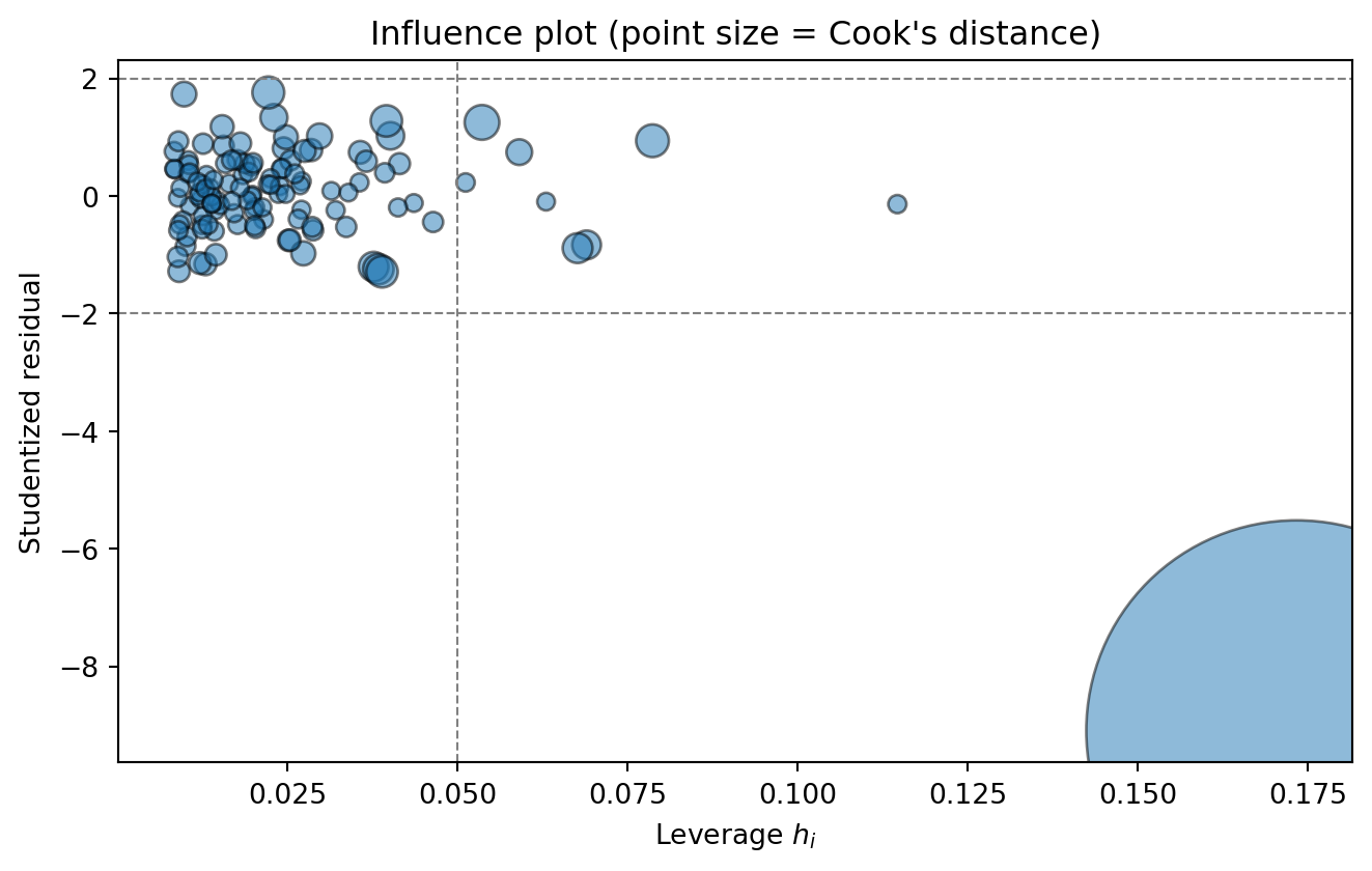
Let’s compute all three diagnostics on our data, after deliberately corrupting one observation:
# Corrupt one observation: unusual X AND a badly wrong Ycorrupt = firms.copy()corrupt.loc[0, "size"] =110# far outside the normal range of firm sizecorrupt.loc[0, "sales"] =40# and a sales figure far below what the model predictsmodel = smf.ols("sales ~ size + adspend", data=corrupt).fit()infl = model.get_influence()diag = pd.DataFrame({"leverage": infl.hat_matrix_diag,"studentized": infl.resid_studentized_internal,"cooks_d": infl.cooks_distance[0],})k =3# intercept + 2 predictorsN =len(corrupt)print(f"Leverage threshold (2k/N) : {2*k/N:.4f}")print(f"Cook's distance threshold (4/N): {4/N:.4f}\n")print("Most influential observations:")print(diag.sort_values("cooks_d", ascending=False).head(5).round(4))plt.figure(figsize=(7, 4.5))plt.scatter(diag["leverage"], diag["studentized"], s=40+4000*diag["cooks_d"], alpha=0.5, edgecolor="k")plt.axhline( 2, ls="--", lw=0.8, color="grey")plt.axhline(-2, ls="--", lw=0.8, color="grey")plt.axvline(2*k/N, ls="--", lw=0.8, color="grey")plt.xlabel("Leverage $h_i$")plt.ylabel("Studentized residual")plt.title("Influence plot (point size = Cook's distance)")plt.tight_layout()plt.show()
Figure 14.1: Influence plot: leverage on the horizontal axis, studentized residual on the vertical axis, and Cook’s distance shown by the size of each point. Dangerous observations sit in the upper-right or lower-right corners.
Observation 0 stands out on every measure: high leverage, a large negative studentized residual, and a Cook’s distance far above the rest. It is exactly the combination that does damage.
Now let’s quantify the damage:
clean_fit = smf.ols("sales ~ size + adspend", data=corrupt.drop(index=0)).fit()comparison = pd.DataFrame({"with the point": model.params,"without the point": clean_fit.params,})comparison["% change"] = (100*(comparison.iloc[:,0]/comparison.iloc[:,1] -1)).round(1)print(comparison.round(4))print(f"\nR-squared with the point : {model.rsquared:.4f}")print(f"R-squared without the point : {clean_fit.rsquared:.4f}")
           with the point  without the point  % change
Intercept         49.9571            33.5304      49.0
size               0.3995             0.7031     -43.2
adspend            1.4795             1.5683      -5.7

R-squared with the point    : 0.4628
R-squared without the point : 0.8171
A single observation out of 120 — less than 1% of the data — cuts the estimated effect of firm size roughly in half and drags R^2 down from 0.82 to 0.46. Nothing else about the dataset changed.
This is the same lesson as the salary example in Chapter 3, now in a regression setting. Least squares minimizes the sum of squared errors, so an observation that is 10 times further from the line than the others contributes 100 times more to the objective function. The fitted line has no choice but to swing toward it. The mean and OLS are both non-robust, and for exactly the same reason: squaring.
14.5 What to do about extreme observations
Here is where judgement matters more than any statistic.
ImportantNever delete an observation just because it is influential
Cook’s distance identifies observations that matter. It does not identify observations that are wrong. Those are entirely different claims, and conflating them is how analysts fool themselves.
Work through this sequence instead:
Investigate. Go back to the raw record. Is it a data-entry error — a misplaced decimal, wrong units, a placeholder like 999 or −1 read as a real value? If so, fix or remove it, and say so in your write-up.
Ask whether it belongs to the population you are studying. A conglomerate in a sample of small retailers, or a merger year in a sample of normal operating years, may be a legitimate observation from a different population. Excluding it is defensible if you define your sample accordingly and state the rule.
If it is real and it belongs, keep it. An influential point that is genuine is telling you something important: your model does not describe the full range of the data. That is a finding about the model, not a defect in the observation. Consider whether a non-linear specification (Chapter 13) or a transformation (Chapter 4) fits the whole range better.
Report both. The most honest approach is often to present results with and without the observation and let the reader see the sensitivity. If your conclusion survives, it is stronger for having been tested. If it does not survive, your reader needed to know that.
Deleting inconvenient data until the p-value cooperates is not diagnostics; it is p-hacking with extra steps.
Robust alternatives are also available when extreme values are genuine but you do not want them dominating the fit:
Winsorization of the independent variables (Chapter 4), which caps rather than deletes.
Robust regression (Huber or M-estimators), which downweights large residuals automatically instead of squaring them.
Log transformation of skewed variables (Chapter 4), which frequently makes the “outlier” disappear entirely — because it was never an outlier on the log scale, only on the original one. This is very often the right answer for business data.
14.6 Heteroskedasticity
Assumption 4 of Chapter 9 requires the error variance to be constant across observations (homoskedasticity). When it is not, we have heteroskedasticity.
This is extremely common in business data, and for an obvious reason: variability usually scales with size. The month-to-month variation in the sales of a multinational is measured in millions; for a corner shop it is measured in hundreds. Plot residuals against fitted values for such data and you get the classic fanning-out cone.
The consequences are worth being precise about:
Coefficients remain unbiased. OLS still estimates the right thing on average.
Standard errors are wrong, so t-statistics, p-values and confidence intervals are all wrong. Typically they are too small, making results look more significant than they are.
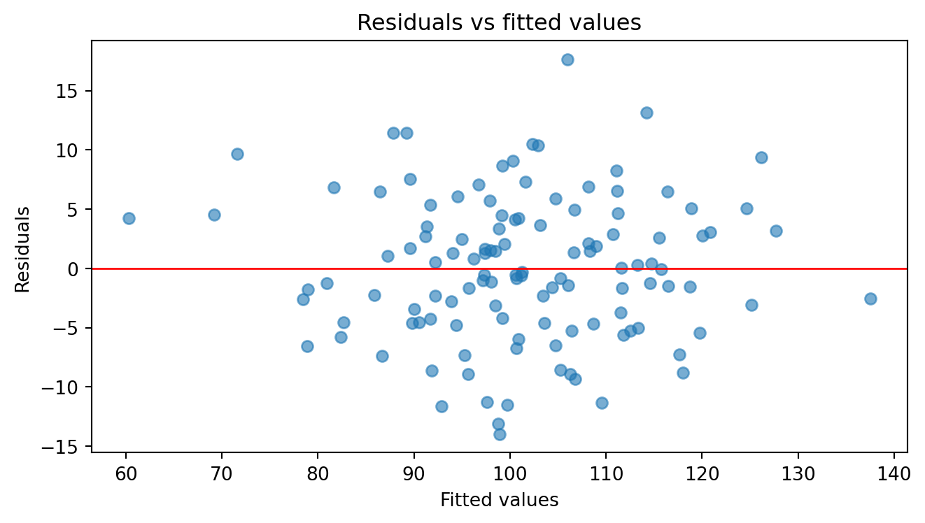
Detection: plot residuals against fitted values and look for a systematic change in spread. Formal tests include Breusch–Pagan and White.
from statsmodels.stats.diagnostic import het_breuschpaganfitted = m_clean.fittedvaluesresid = m_clean.residplt.figure(figsize=(7, 4))plt.scatter(fitted, resid, alpha=0.6)plt.axhline(0, color="red", lw=1)plt.xlabel("Fitted values")plt.ylabel("Residuals")plt.title("Residuals vs fitted values")plt.tight_layout()plt.show()bp = het_breuschpagan(resid, m_clean.model.exog)print(f"Breusch-Pagan statistic = {bp[0]:.3f}, p-value = {bp[1]:.4f}")print("H0: the errors are homoskedastic (constant variance).")
Figure 14.2: Residuals versus fitted values — the single most useful diagnostic plot in regression.
Breusch-Pagan statistic = 0.125,  p-value = 0.9396
H0: the errors are homoskedastic (constant variance).
A residuals-versus-fitted plot should look like a structureless horizontal band. Any pattern is a message:
Pattern in the plot
What it means
Remedy
Random horizontal band
Assumptions look fine
Nothing to do
Cone / fan shape
Heteroskedasticity
Robust standard errors, or log-transform Y
Curved (U or inverted-U)
Missing non-linear term
Add a quadratic term (Chapter 13)
Wave or cycles over time
Autocorrelation
Time-series methods (Chapter 15)
Remedies: the modern default is to use heteroskedasticity-robust standard errors (White or Huber–White standard errors), which correct the inference without changing the coefficients. In statsmodels this is a single argument:
Comparing the two standard error columns is itself a useful diagnostic: if they are close, heteroskedasticity is not a practical concern; if they diverge materially, report the robust ones. Since robust standard errors cost nothing when the errors are in fact homoskedastic, many practitioners simply use them by default.
The other classical remedy is to transform the dependent variable. Taking logs of a variable whose spread grows with its level converts multiplicative variation into additive variation — which is precisely the homoskedasticity assumption. This often fixes heteroskedasticity, non-normality and outliers simultaneously, which is why the log transformation of Chapter 4 is such a workhorse.
14.7 Autocorrelation
Assumption 5 requires the errors to be uncorrelated with each other. In time-series data they very often are not: if the model underpredicts this month, it tends to underpredict next month too. This is autocorrelation (or serial correlation).
Like heteroskedasticity, it leaves coefficients unbiased but corrupts standard errors — usually understating them, which inflates significance.
The classical detection tool is the Durbin–Watson statistic, which ranges from 0 to 4:
DW \approx 2: no autocorrelation
DW < 2: positive autocorrelation (the common case)
DW > 2: negative autocorrelation
from statsmodels.stats.stattools import durbin_watsonprint(f"Durbin-Watson = {durbin_watson(m_clean.resid):.3f}")print("Values near 2 indicate no autocorrelation.")
Durbin-Watson = 1.663
Values near 2 indicate no autocorrelation.
Values roughly between 1.5 and 2.5 are usually considered acceptable. The remedies — Newey–West standard errors, lagged dependent variables, and differencing — belong to time-series regression and are developed in Chapter 15.
14.8 A diagnostic checklist
Rather than treating these as isolated tests, run them as a routine after estimating any regression:
Plot residuals versus fitted values. One plot detects non-linearity, heteroskedasticity, and gross outliers. If you do only one diagnostic, do this one.
Check the VIFs — but only act on them if you care about interpreting a specific collinear coefficient.
Compute Cook’s distance and look at the largest handful of observations. Investigate them as data, not as statistics.
Compare classical and robust standard errors. If they differ materially, report the robust ones.
For time-series data, check the Durbin–Watson statistic and plot the residuals against time.
Ask what is missing. No diagnostic in this chapter can detect omitted variable bias, which is the most serious problem of all. Only subject-matter knowledge can. Before trusting a coefficient, ask: what else could plausibly drive both my X and my Y?
That last point deserves emphasis, because it is the boundary of what statistics can do for you. Every technique in this chapter checks whether the model is internally consistent with its own assumptions. None of them can tell you whether you asked the right question or measured the right variables. That remains the analyst’s job — which is why this book began with two chapters on business strategy and financial analysis rather than with statistics.