Financial analysis is the selection, evaluation and interpretation of the financial and market data of a firm, most of which is contained in its financial statements. Financial statements convey information about two distinct things:
Operational performance — how efficiently the firm uses its assets to generate a return on the money invested in it.
Financial condition — the firm’s ability to satisfy its debt obligations on time.
Keeping these two questions separate is the key to reading financial statements well. A firm can be highly profitable and still go bankrupt because it runs out of cash; a firm can be perfectly solvent and still destroy shareholder value.
The three main financial statements are a) the balance sheet, b) the income statement, and c) the statement of cash flows.
The main types of financial analysis are:
Financial ratio analysis
Cash flow analysis
This chapter focuses on financial ratio analysis. Before reviewing the ratios we need to review the statements they are built from, so the next sections describe the main elements of each statement, and then we examine the ratios themselves.
NoteWhy a statistics book starts with accounting
Financial statements are the raw data of business analytics. Almost every variable we will model in later chapters — sales growth, profitability, leverage, returns — is either taken directly from a financial statement or computed from one. If the definitions are fuzzy, the models built on them will be fuzzy too. It is also worth noticing that essentially all of these variables are strongly right-skewed across firms, which is exactly the situation Chapter 3 warns us about.
2.2 Review of financial statements
The three statements answer three different questions:
The three financial statements at a glance
Statement
Question it answers
Time reference
Balance sheet
What does the firm own and owe?
A point in time (a snapshot)
Income statement
How much wealth did the firm generate?
A period (a movie)
Cash flow statement
Where did the cash come from and go?
A period (a movie)
2.2.1 Balance Sheet
The balance sheet is a statement that reports the book value of all firm assets along with all firm liabilities and shareholder equity. A firm asset is any resource the company acquires in order to operate and generate revenue and firm earnings. A firm liability is any payment commitment of the firm. A liability can be financial debt or accounts payable (e.g. when a firm acquires raw material and will do the corresponding payment later). Shareholder equity is the book value of a) the original amount of money invested by shareholders (common equity), and b) the cumulative retained firm earnings over time.
In other words, a firm obtains resources (total assets) from only two possible places: from its owners and its own accumulated operations (shareholders’ equity), or from creditors such as banks and suppliers (total liabilities). The left-hand side answers what the firm has; the right-hand side answers who has a claim on it. They are equal by construction — every peso of resource had to come from somewhere.
For assets, liabilities and shareholders’ equity, the firm reports several accounts. Asset accounts include cash, accounts receivable, inventory, and gross plant and equipment; liability accounts include accounts payable, short-term debt and long-term debt. In the balance sheet the firm reports the book value of each account, which accumulates from the day the firm started operations up to the reporting date. This is why the balance sheet has only an ending date rather than a period: it is a stock, not a flow. It is normally presented alongside the comparable figure from one year earlier.
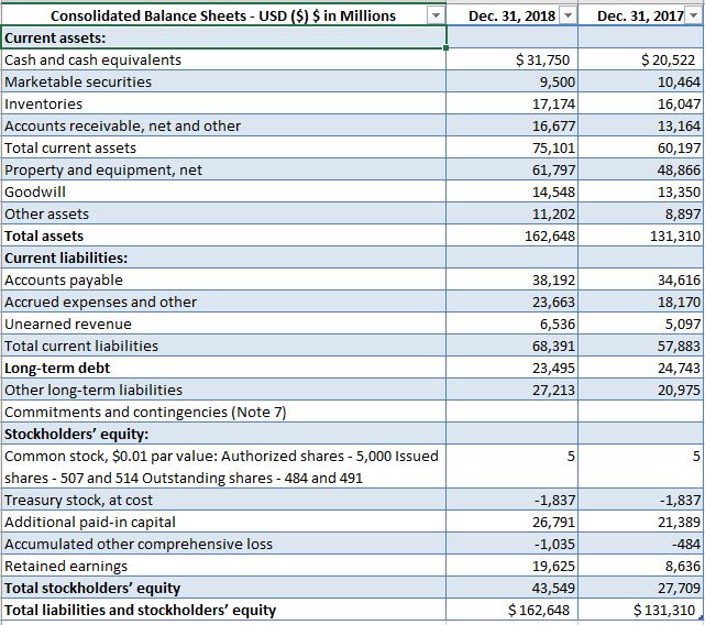
Below is the real balance sheet of Amazon for 2018. 1
2018 Amazon balance sheet summary
Amazon’s total assets increased by about 24% in 2018 while total liabilities increased by about 15%. Since assets grew faster than liabilities, equity must have grown fastest of all — the accounting equation guarantees it. That single comparison already tells us that Amazon financed its 2018 growth mostly out of retained earnings rather than new debt.
2.3 Income statement
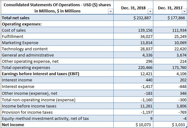
If the balance sheet is a photograph, the income statement is a film of the firm’s productivity over a specific time period. Public firms must report financial statements each quarter (every 3 months) plus an annual report. The income statement shows how much the firm sold and every category of expense, all the way down to the net income of the period. Net income is the economic wealth generated during the period. Here is Amazon’s 2018 income statement:
2018 Amazon income statement summary
In 2018 Amazon grew strongly and increased net income even faster. Sales rose by about 31%, while net income rose by about 232% — that is, net income more than tripled. This is an outstanding result for a firm of that size, and the gap between the two growth rates is itself informative: net income growing seven times faster than sales means margins expanded sharply, not merely that the firm sold more.
2.4 Cash flow statement
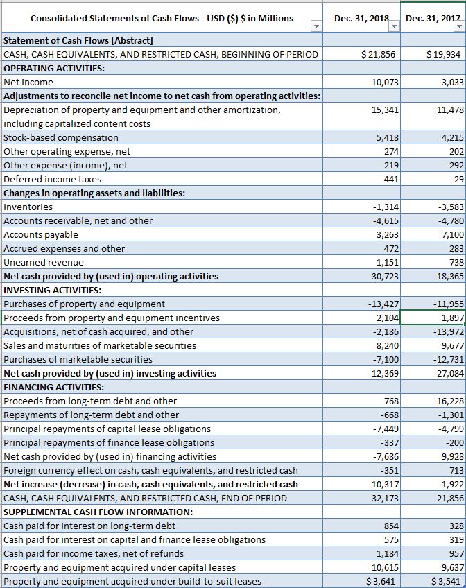
The cash flow statement shows how the firm generates and uses cash across three types of activity: operating, investing and financing. Cash flow differs from net income for two reasons: accruals (revenue is recorded when the sale is made, not when the customer pays, and the same applies to expenses) and non-cash expenses such as depreciation. This is why a growing, profitable firm can still run out of cash — profit is an opinion about timing, cash is a fact. Here is Amazon’s 2018 statement of cash flows:
2018 Amazon cash flow statement summary
Amazon increased cash flow from operations by 67%, from $18,365 million in 2017 to $30,723 million in 2018. Note that this figure is roughly three times its net income for the year — the gap is mostly depreciation and favourable working-capital timing, and it is precisely the kind of discrepancy that a ratio analysis based only on the income statement would miss.
2.5 Elements of Financial Statements
I focus only on the basic elements of the financial statements. This is not a comprehensive list, but it covers everything needed to compute the main financial ratios. It is worth learning this notation carefully, because the rest of the chapter is essentially algebra applied to these symbols.
Balance sheet variables — assets:
Symbol
Meaning
TA
Total assets
CASH
Cash and cash equivalents
AR
Accounts receivable (A/R)
INV
Inventories
CA
Current assets
GPEQ
Gross plant and equipment — the fixed assets of the company
ADEP
Accumulated depreciation — subtracted from GPEQ, since it records how much the fixed assets have been used up
NFA
Net fixed assets = GPEQ − ADEP
Balance sheet variables — liabilities and shareholders’ equity:
Symbol
Meaning
TL
Total liabilities
AP
Accounts payable (A/P)
CL
Current liabilities, including short-term debt
LTD
Long-term debt
CS
Common stock
PS
Preferred stock
CRE
Cumulative retained earnings
SHE
Book value of shareholders’ equity = CS + PS + CRE
Income statement variables:
Symbol
Meaning
S
Total sales (revenue)
COGS
Cost of goods sold
SGAE
Selling, general and administrative expenses
DEP
Depreciation and amortization of the period
EBIT
Earnings before interest and taxes
IE
Interest expense
EBT
Earnings before taxes
T
Taxes
NI
Net income
DIV
Dividends paid
RE
Retained earnings of the period = NI − DIV
WarningStocks versus flows
Balance sheet variables are stocks: accumulated amounts measured at a single date. Income statement variables are flows: amounts generated during a period. Almost every financial ratio divides a flow by a stock (ROA = NI / TA, for instance), which is why the convention of using beginning-of-period assets matters — you want the resources that were available to generate the flow, not the resources you ended up with after generating it. Mixing stocks and flows carelessly is the most common source of wrong ratios.
Let us now use simple algebra to make the relationships between these elements explicit. The main equation of accounting is:
TA_{t}=TL_{t}+SHE_{t}
TA_{t} = Total assets: the book value of all resources the company owns at the end of period t.
TL_{t} = Total liabilities: the total value of debt (short-term and long-term debt plus current liabilities such as accounts payable).
SHE_{t} = Book value of shareholders’ equity: the capital investors have contributed to the firm — common stock (CS) and preferred stock (PS) — plus cumulative retained earnings (CRE):
SHE_{t}=CS_{t}+PS_{t}+CRE_{t}
CS_{t}=Book value of common stock at period t
PS_{t}= Book value of preferred stock at period t
CRE_{t} = Cumulative retained earnings
The retained earnings of a single period equal net income minus the dividends paid in that period.
So a firm has exactly three sources of resources: a) TL — financing from creditors and suppliers, b) CS + PS — capital contributed by investors, and c) CRE — cumulative profits from business operations that were reinvested rather than distributed:
TA_{t}=TL_{t}+(CS_{t}+PS_{t})+CRE_{t}
CRE_{t}=CRE_{t-1}+RE_{t}
RE_{t}=NI_{t}-DIV_{t}
Now, looking closer to both Total Assets and Total Liabilities, we can see that:
TA_{t}=CA_{t}+NFA_{t}
NFA_{t}=GPEQ_{t}-ADEP_{t}
CA_{t}=CASH_{t}+AR_{t}+INV_{t}
TL_{t}=CL_{t}+LTD_{t}
Now, let’s analyze in detail the relationship of the income statement variables:
EBIT_{t}=S_{t}-COGS_{t}-SGAE_{t}-DEP_{t}
DEP_{t} represents the depreciation of tangible assets and the amortization of intangible assets during period t. Depreciation measures how much of the asset was consumed in the period. It is a non-cash expense: it reduces earnings without any money leaving the firm, which is exactly why cash flow and net income diverge.
So net income equals sales, minus cost of goods sold (mostly variable costs), minus selling and administrative expenses (mostly fixed costs), minus depreciation, minus interest expense, minus taxes.
At the end of each year, if the firm generated positive net income, management must decide whether to pay dividends to shareholders or retain the money. Dividends are paid out of the net income generated in the period; whatever is left is reinvested in the firm and is called retained earnings. The retained earnings of the period are added to cumulative retained earnings, which is part of shareholders’ equity.
This is the crucial link: the income statement and the balance sheet are connected through net income. Net income is a flow that, once dividends are subtracted, flows into the equity stock on the balance sheet.
We can conceptualize a firm as an engine with the potential to generate economic wealth measured in future cash flows. These cash flows must be able to satisfy:
• The required rate of return of the firm shareholders, and
• The debt rate of creditors
In other words, after a period, the firm must be able to generate wealth from its operations to first cover the financial debt with creditors, and then, the expected dividends (or return) that shareholders require. However, before paying creditors and shareholders, the firm also has to reserve cash flows to invest in fixed assets in order to expand or grow, and also it has to reserve some resources for working capital for the following period.
Working capital refers to the short-term liquidity and operational efficiency. Working capital is the difference between current assets and current liabilities. Then, we can visualize the different cash flows generated by a firm in a period as follows:
\underbrace{CFO - \Delta NWC - CAPEX}_{\text{what the firm generates and keeps free}} = \underbrace{CF_{\text{creditors}} + CF_{\text{shareholders}}}_{\text{what is claimed by capital providers}}
In words: cash flow from operations, minus cash invested in working capital, minus cash invested in capital expenditure, must equal the cash flow paid to creditors plus the cash flow paid to shareholders.
This is called the cash flow identity, and it is an identity in the strict sense — it holds by construction, not as an approximation. The intuition is simply that every peso the business generates must end up somewhere: reinvested in the business, or handed to someone with a claim on it.
In the following section I decompose the accounting equation to derive this identity and show exactly why it holds.
2.6 Cash flow identity
I will examine in detail the main equation of accounting to identify all different types of cash flows generated by the firm. To keep the analysis simple, I will assume that the total revenue of the firm comes from the core business operations and not from other activities such as financing or investing activities. I start with the main accounting equation:
TA_{t}=TL_{t}+SHE_{t}
Total assets, total liabilities and shareholders’ equity are as follows:
Now I can subtract the same figures but from the previous accounting period in order to get changes for each amount:
\left(CA_{t}+NFA_{t}=\left[CL_{t}+LTD_{t}\right]+\left[CS_{t}+PS_{t}+CRE_{t}\right]\right)-\left(CA_{t-1}+NFA_{t-1}=\left[CL_{t-1}+LTD_{t-1}\right]+\left[CS_{t-1}+PS_{t-1}+CRE_{t-1}\right]\right)
Then, I get:
This detailed decomposition of the financial statement items leads to an important conclusion: creditors and shareholders have a claim on cash flow from operations only after the firm has invested in the working capital and the capital expenditure it needs to stay in business. This is the foundation of the concept of free cash flow, which is the basis of essentially every valuation model in corporate finance.
TipWhy this derivation is worth the effort
We could have simply asserted the cash flow identity. Deriving it from the accounting equation shows that it is not a convention someone invented — it follows necessarily from the fact that assets equal liabilities plus equity in every period. When a relationship in finance is an identity, no empirical test can refute it, and any dataset in which it fails contains a data error. That is a useful thing to know before you start modeling.
2.7 Financial ratio analysis
A ratio is a division between two numbers, and it conveys information about the relationship between two variables. A financial ratio can be any division between two variables taken from the financial statements. The reason ratios are so useful is scale invariance: absolute figures are incomparable between a corner shop and a multinational, but a 12% profit margin means the same thing in both.
We classify financial ratios into five groups, each answering a different question:
The five families of financial ratios
Group
Question it answers
Profitability
How much of each peso of sales becomes profit?
Return on investment
How much profit does each peso of invested capital generate?
Financial leverage
How much of the firm is financed with debt, and can it service that debt?
Liquidity
Can the firm meet its short-term obligations?
Activity
How intensively are the firm’s assets being used?
Besides these ratios, a simple and very effective way to evaluate operating performance and financial condition is to express the financial statements as percentages. In the balance sheet, every item is expressed as a percentage of total assets; in the income statement, as a percentage of total sales. These are called common-size financial statements.
WarningA ratio is a comparison, never a verdict
A ratio in isolation means almost nothing. “Current ratio = 1.4” is neither good nor bad until you compare it against (a) the same firm in previous periods, (b) competitors in the same industry, or (c) an accepted benchmark. Industry matters enormously: a supermarket operates comfortably with a current ratio below 1 because it sells for cash and pays suppliers late, while a shipbuilder cannot. Every ratio in this chapter should be read as the start of a question, not the end of one.
2.8 Return on Investment and profitability Ratios
Now let’s play with these variables to create financial ratios that convey information about return on investment. If I were one of the main investors of a firm, I would like to see how productive the firm is utilizing its assets, and then, how much I would make from my investment. Then, I would be interested in the following ratios:
ROA_{t}=\frac{NI_{t}}{TA_{t-1}}
ROABIT_{t}=\frac{EBIT_{t}}{TA_{t-1}}
Note: the use of t-1 is optional and it depends on the specific analysis. Many analysts compute ROA of t using assets of the previous period (t-1). ROA and ROABIT are measures of return on assets. In other words, both convey information about what percentage represents earnings with respect to the total book value of its assets. ROABIT is also known as “Basic earnings power”. The decision about which of these two measures is the best to represent return on assets depends on the specific context and also specific information to be analyzed.
A simple measure of operational efficiency is asset turnover (ATO), which is how often or how fast the assets of the firm are generating revenues:
ATO_{t}=\frac{S_{t}}{TA_{t-1}}
Learning about the ROA can give investors an idea about how efficient the company is using its assets. However, if an investor observes an increase of ROA from one year to another, he or she will not know what is the source of this improvement. ROA can change due to changes in profit margin or asset efficiency. Let’s do simple math to identify two components of ROA. If we multiply the ROA components by the ratio S/S, which is equal to one:
Now we get 2 components of ROA, that is Profit Margin and Asset Turnover.
\frac{NI_{t}}{S_{t}}=Profit\,Margin
\frac{S_{t}}{TA_{t-1}}=Asset\,Turnover
So ROA = (\text{Profit margin}) \times (\text{Asset turnover}). This is the core of the DuPont system, a decomposition developed at the DuPont corporation in the early twentieth century and still in daily use.
The net profit margin is the percentage of sales that ends up as profit. To see why the decomposition is useful, suppose last year’s ROA was 0.20 and this year’s is 0.10. The ROA alone tells us performance halved; it does not tell us why. The decomposition does. The decline must come from a fall in profit margin (costs rose or prices fell), from a fall in asset turnover (sales stagnated or the asset base grew), or from both. Consider two scenarios that produce exactly the same 0.10 ROA:
Last year
Scenario A
Scenario B
Profit margin
10%
5%
10%
Asset turnover
2.0
2.0
1.0
ROA
20%
10%
10%
In Scenario A the firm has a margin problem: it is selling just as much per peso of assets but keeping half as much of each sale. Management should look at pricing, input costs, or the product mix. In Scenario B the firm has a turnover problem: margins are intact, but the asset base is no longer producing sales — perhaps a new plant was built and has not yet come online, or inventory and receivables have ballooned. These two situations call for entirely different responses, and the undecomposed ROA cannot distinguish them.
This is the same lesson as the DuPont example in Chapter 1, and it is a lesson that generalizes far beyond finance: an aggregate measure describes; a decomposed measure diagnoses.
Another important ratio for investors is the return on equity - maybe the most important for them. ROE is simply:
ROE_{t}=\frac{NI_{t}}{SHE_{t}}
Now let’s work with EBIT instead of NI, to see in more detail the role of financing (IE) and taxes (T) in the bottom line. Recall the definition of ROA before interest and taxes:
ROABIT_{t}=\frac{EBIT_{t}}{TA_{t-1}}
Doing simple math with the ratios and the income statement rules:
NI_{t}=EBIT_{t}-IE_{t}-T_{t}
If we consider a Tax Rate TR, then we can express NI as:
The term \left(EBIT_{t}\right)\left(1-TR_{t}\right) is a version of “unlevered” earnings — what the firm’s after-tax earnings would have been with no debt financing at all, since without debt the interest expense is zero. I will call it unlevered net income.
The term \left(IE_{t}\right)\left(TR_{t}\right) enters the formula with a positive sign, meaning it adds to net income. This is the famous interest tax shield: because interest is deductible before taxes, each peso of interest paid reduces the tax bill by TR pesos. I will call this term the tax benefit.
So debt financing brings two distinct benefits: the tax shield, and the ability to put more resources to work in the productive activities of the firm. Remember that total assets equal shareholders’ equity plus total liabilities, so both short-term and long-term debt expand the resource base the firm uses to generate earnings.
Of course, interest expense also reduces net income directly, as the formula shows. But debt is often cheaper than equity — creditors bear less risk than owners, so they demand a lower return. The condition for debt to create value is that the return the firm earns on the borrowed money exceeds the after-tax interest rate paid on it.
NoteA numerical look at the tax shield
Take a firm with EBIT = 1{,}000 and a tax rate of 30%.
No debt
With $200 of interest
EBIT
1,000
1,000
Interest expense
0
200
EBT
1,000
800
Taxes (30%)
300
240
Net income
700
560
Net income falls by 140, not by the full 200 of interest. The missing 60 is the tax benefit: IE \times TR = 200 \times 0.30 = 60. The government effectively pays 30% of the firm’s interest bill.
In practice, most firms borrow simply because they lack the cash to start or continue operations. But entrepreneurs should be aware that debt also carries these structural advantages. If you had enough cash to launch your company, it can still be worth borrowing if you can access a reasonable interest rate — and even at a high rate, if you believe the business can grow fast enough to capture a market opportunity that would otherwise be lost. The trade-off, discussed in the next section, is that debt payments are compulsory while dividends are not.
Now, I continue playing with return on investment ratios to examine the components of earnings:
Then, we can say that ROA can also be expressed as Net Income share of owners’ equity after taxes times ROA Before Interest and Taxes. Now we can decompose the second factor multiplying and dividing by Sales in order to identify operating margin and asset turnover:
Unlike Profit Margin, Operating Margin is a percentage of sales that the firm is generating as earnings from operations without considering firm ownership structure (debt/equity ratio) neither tax expenses. Then Operating Margin can also be analyzed when tracking ROA over time.
Both profit margin and operating margin are known as profitability ratios.
Now I will work with return on investment from the investors perspective -ROE. If I multiply ROE times TA and divide it by TA:
So ROE equals profit margin times asset turnover times TA/SHE. This last term is a measure of financial leverage known as the equity multiplier. If the firm carries no debt, then SHE = TA and the multiplier equals exactly 1; the more the firm borrows, the larger it grows. This is the three-factor DuPont decomposition:
It says that a firm can raise the return it delivers to its owners in three, and only three, ways: earn more on each sale, sell more with the same assets, or finance the same assets with less of its owners’ money.
There is a subtlety worth pausing on. The formula seems to say that ROE rises mechanically with the equity multiplier — so why does no firm borrow infinitely? Because the three factors are not independent. More debt means more interest expense, which reduces net income and therefore the profit margin. Leverage improves ROE only while the extra return earned on the borrowed assets exceeds the after-tax cost of the debt. Beyond that point the margin effect dominates and ROE falls, on top of the increased risk of financial distress. Let us now look at leverage ratios in more detail.
2.9 Financial leverage ratios
Now, assuming that the firm has access to long-term debt, then:
TA_{t}=SHE_{t}+LTD_{t}+CL_{t}
This means that a company can finance its asset with either debt or equity. Now, we can do the following simple math to explore financial leverage ratios:
SHE_{t}=TA_{t}-\left(LTD_{t}+CL_{t}\right)
Now dividing all terms by the book value of shareholders’ equity:
Since total liabilities are long-term debt plus current liabilities, TL_t = LTD_t + CL_t, this simplifies to:
\frac{TA_{t}}{SHE_{t}}=1+\frac{TL_{t}}{SHE_{t}}
\frac{TL_{t}}{SHE_{t}} is a more direct measure of financial leverage: the more the firm borrows, the higher this ratio, and therefore the higher the equity multiplier. The equation shows they are not two independent measures but the same measure shifted by one.
Other measures of financial leverage are the ratio of debt to equity and the ratio of debt to assets:
\frac{LTD_{t}}{SHE_{t}} = debt to equity ratio
\frac{LTD_{t}}{TA_{t}} = debt to assets ratio
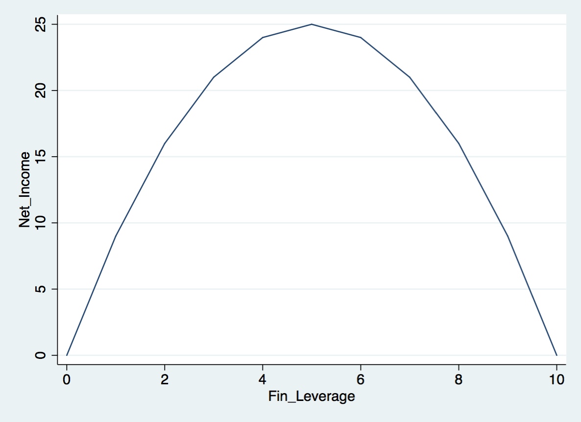
The interesting question is: what is the best degree of financial leverage? There is no universal answer. It depends on external factors (macroeconomic conditions, interest rates, industry volatility) and internal ones (the cost of equity, the stability of cash flows, the tangibility of the assets that can serve as collateral). What we can say is that leverage plausibly has an inverted U-shaped effect on shareholders’ wealth: up to some point, the tax shield and the expanded asset base dominate; beyond it, the cost of financial distress dominates. For each firm there is an expected optimal leverage, and moving away from it in either direction destroys value. Although the true relation is not exactly quadratic, we can visualize it as:
Expected effect of leverage on firm net income
Note
This inverted-U is our first encounter with a non-linear relationship between two business variables, and it is a good one to remember. A linear regression of firm value on leverage would find a coefficient close to zero — not because leverage does not matter, but because its effect is positive on one side of the optimum and negative on the other, and the two cancel out. Chapter 13 shows how to model relationships of this shape properly.
Debt financing obliges the company to pay principal and interest on a fixed schedule. Equity financing carries no such obligation: the board decides when and how much to pay as dividends, and a firm that needs resources to grow can simply suspend the dividend. It cannot suspend a debt payment. This asymmetry is the essence of financial risk: debt converts a variable claim into a fixed one, which magnifies both good and bad outcomes for the residual owners.
To examine financial risk in more detail we look at ratios based on interest expense. The higher the interest burden relative to earnings, the harder it is to make principal and interest payments. These are known as coverage ratios.
This ratio says how many times over the firm could pay its interest bill out of operating earnings. The higher it is, the safer the debt. A firm with an interest coverage of 8 can absorb a severe drop in earnings and still service its debt; a firm at 1.2 is one bad quarter away from default.
This ratio ignores other fixed commitments, most importantly lease expenses. Leases resemble interest in that the company is obliged to make fixed payments over a set period. Since lease expenses are already deducted within EBIT as a fixed cost, we add them back to both numerator and denominator:
This ratio is usually lower than the interest coverage ratio and gives a more complete picture of the firm’s ability to meet all of its fixed financial commitments, not just the ones labelled “debt”.
A third coverage ratio replaces earnings with actual cash:
Interest and tax expenses are added back to cash flow from operations so that the numerator measures the cash available before paying interest — otherwise we would be asking whether the firm can pay interest out of money it has already used to pay interest.
Why is EBIT not enough for assessing financial risk? Because creditors are paid in cash, not in earnings. Cash flow from operations accounts for how much the firm is financing from its suppliers (accounts payable) and how much its customers are financing from the firm (accounts receivable), and it excludes depreciation, which reduces EBIT without consuming any cash. A firm can report healthy EBIT while its cash is locked up in receivables from customers who are not paying. That firm’s interest coverage ratio looks fine, and its cash flow coverage ratio does not.
2.10 Liquidity ratios
Where leverage ratios measure the company’s ability to meet long-term obligations, liquidity ratios measure its ability to meet short-term ones — using not just cash but every asset that can readily be converted into cash. These are the liquid or current assets. Subtracting current liabilities from current assets gives net working capital, the pool of resources that funds day-to-day operations. If NWC = net working capital:
NWC=CA-CL
Since net working capital funds day-to-day operations, we need to know how long those operations take to turn cash back into cash. This is the operating cycle: the time between paying for inputs and collecting the money from the resulting sales. It is usually composed of the following phases: a) purchase raw materials, b) produce goods or services, c) pay for the inventory, d) sell the goods or services, e) extend credit to customers through accounts receivable, and f) collect cash from direct sales and from accounts receivable.
The longer the operating cycle, the more net working capital the company needs, because more of its money is tied up in the cycle at any moment. So how do we measure it?
2.10.1 Operating cycle
The operating cycle is the time a company takes to produce goods, store them, sell them, and finally collect the cash. Equivalently: the time between the cash going out to buy raw materials and the cash coming back in from customers. This concept applies mainly to manufacturing and commercial companies that hold inventory.
To provide an estimate of the operating cycle of the company we can think in two sub-cycles: 1) how long it takes to the company to sell 100% of its average inventory, and 2) how long it takes to the company - on average - to collect cash from sales. The first sub-cycle is also known as days sales in inventory, while the second sub-cycle is also known as the days of credit. This is a rough but acceptable estimate of the actual operating cycle. Then, let’s analyze these two sub-cycles.
2.10.2 Days sales in inventory
The inventory in the annual balance sheet represents the cost of goods “not” sold yet. Then, we can take this amount and divide it by the cost of good sold (COGS) at the end of the year. This will represent the proportion of goods that are not sold with respect to the goods sold during the year
\frac{Inventory_{t}}{COGS_{t}}= Proportion of goods not sold with respect to goods sold
Considering that these amounts are annual amounts, then we can translate this proportion in terms of the proportion of the year it takes to sell all the inventory if we assume that the company regularly produces and sells goods during the whole year, and also that the inventory level at the end of the year represents inventory levels during the year. Then, the number of days the company takes - on average - to sell all its inventory can be estimated by:
\frac{Inventory_{t}}{COGS_{t}}*365= Days sales in inventory=DSI
Now since most of the companies tend to select an end period with the lowest level of inventory during the year, this sub-cycle will be underestimated. It would be more accurate to calculate the average inventory of the last 4 quarters of the year instead of the last inventory of the year.
2.10.3 Days on credit
Days of credit is the average number of days the company takes to collect cash from sales. To easily estimate this sub-cycle we can assume that all sales are credit sales, but we do not have detailed information about how often our customers make their payments. However, we can estimate this by looking at accounts receivable. Then we can look at the proportion of accounts receivable with respect to credit sales - sales in this case. This proportion gives us a measure of how fast the company is collecting cash.
\frac{AR_{t}}{S_{t}}= Proportion of accounts receivable with respect to credit sales
Then, if we multiply this proportion by 365 we can get the average number of days the firm takes to collect cash from sales:
\frac{AR_{t}}{S_{t}}*365 = Days on credit=DOC
Now we can get the estimate of operating cycle by adding Days sales in inventory and Days on credit:
Once we have a proxy (measure) of the operating cycle, then we have an idea how long the company takes to generate cash from operations. This can help managers to decide which would be a good level of net working capital to make sure that the firm will not run out of cash and will not affect day-to-day operations. For example, if a company has an operating cycle of about 90 days, this means that it is strongly recommended to always have net working capital equivalent to cover 3 months of operations - including fixed and variable costs.
2.10.4 Cash conversion cycle
Now, considering that the company can take advantage of “free” financing from suppliers when buying on credit, then we can also estimate the an average number of days the company pays its accounts payable. If we put this credit cycle together with the operating cycle (subtracting credit cycle days from operating cycle days), we can get an estimate of number of days the company takes to convert or generate cash from operations considering not only the credit we give to our customers, but also the credit we get from our suppliers. This net cycle is known as cash conversion cycle (CCC).
To estimate the cash conversion cycle, we need to estimate the cycle for accounts payable, also know as days payable outstanding (DPO). We can follow the same logic we use to estimate the days on credit, assuming that all purchases are made on credit. Since we do not have detailed information about the value of all purchases and how much was on credit, we can use cost of good sold minus depreciation (of operating equipment) as the total value of credit purchase. Then, we can estimate the DPO as:
DPO indicates how many days, on average, the company takes to pay its accounts payable. Subtracting these days from the operating cycle gives a “net” cycle of cash generation, known as the cash conversion cycle:
The cash conversion cycle can also be used to set minimum levels of net working capital, although the operating cycle is the more conservative benchmark for that purpose.
TipThe cash conversion cycle as a strategy
A negative cash conversion cycle means the company collects from its customers before it pays its suppliers — so growth generates cash instead of consuming it. This is not an accounting curiosity; it is a business model. Large retailers and marketplace platforms sell inventory in days, take cash immediately, and pay suppliers 60 or 90 days later. Their suppliers are, in effect, financing their growth at zero interest.
The strategic point is that CCC is not a passive measurement. Reducing DSI (faster inventory turnover), reducing DOC (faster collection), and increasing DPO (slower payment to suppliers) are three concrete levers management can pull, and each corresponds to a different operational initiative.
2.10.5 Liquidity ratios
We now turn to the ratios that convey the ability of a company to meet its short-term obligations: the current ratio, the quick ratio, and the net working capital-to-sales ratio.
\text{Current ratio} = \frac{CA_{t}}{CL_{t}}
This measures the firm’s ability to cover its current liabilities with its current assets. In theory current assets convert into cash within a year — but “within a year” may be far too slow if an obligation falls due next month, which is why we also want a more conservative measure. The quick ratio (or acid-test ratio) removes inventory, typically the slowest current asset to convert into cash:
The gap between these two ratios is itself informative: a large gap means the firm’s apparent liquidity depends heavily on selling inventory, which is exactly what becomes hard to do in a downturn.
Finally, the net working capital-to-sales ratio expresses liquidity relative to the scale of the business:
\text{NWC-to-sales ratio} = \frac{NWC_{t}}{S_{t}}
This tells the company how many cents of net working capital it must hold for each peso of sales. The longer the operating cycle, the larger the net working capital required and the larger this ratio — which means it should grow proportionally as the firm grows. Many fast-growing firms fail precisely here: sales expand, working capital needs expand with them, and the firm runs out of cash while its income statement looks excellent.
Days sales in inventory and days of credit tell us how liquid inventory and receivables are individually; the liquidity ratios tell us the firm’s overall ability to meet short-term obligations, with and without relying on inventory.
2.10.6 Activity ratios
Activity ratios measure the productivity of specific assets — inventory, accounts receivable, total assets. They are expressed as the number of times the company turns over the asset during the period (a year or a quarter, depending on the statement used). Note that activity ratios and the day-based cycle measures above are two views of the same thing: turnover = 365 / days.
2.10.6.1 Inventory turnover ratio
The inventory turnover ratio measures how many times a year the company sells its inventory:
\frac{COGS_{t}}{Inventory_{t}}= Inventory turnover ratio
For example, an inventory turnover of 3 computed from an annual income statement means the company sells and replaces its entire inventory 3 times a year, on average. This is the mirror image of days sales in inventory: inventory turnover is simply 365 / DSI. If turnover is 3, then DSI = 365/3 \approx 122 days.
Interpretation is highly industry-dependent. A supermarket may turn over its inventory 15 or 20 times a year; a jeweller may turn it over twice. Neither number is good or bad in isolation — but a supermarket at 2 would be in serious trouble.
2.10.6.2 Accounts receivable turnover
Accounts receivable turnover measures how many times a year the company collects its credit sales. Assuming that the accounts receivable at the end of the year is representative throughout the year, and assuming that 100% of the sales are on credit, then we can estimate the accounts receivable turnover dividing net credit sales by account receivable:
\frac{NetCreditSales_{t}}{AR_{t}}=Accounts receivable turnover ratio
NetCreditSales_{t}=S_{t}-SalesReturns_{t}
For example, if this ratio is equal to 15 times, then it means that the company collects cash from credit sales 15 times a year. This ratio indicates how effectively a company is using credit extended to customers. There is a risk of extending credit to customers since there is always the possibility of default (the fact that some credit sales will never be paid).
Looking at the “Days of credit” formula, we can see that Days of credit can be estimated just by dividing 365 by the accounts receivable turnover ratio (assuming that there is no Sales returns). In other words, if we consider 365 days in the year and the company collects cash from credit sales 15 times a year, this means that the company takes about 24 days (365/15) to collect cash from credit sales.
2.10.6.3 Total asset turnover
We already met this ratio in the DuPont analysis of return on assets. It indicates how many pesos of sales the company generates per peso of assets in the year:
ATO = \frac{S_{t}}{TA_{t}}
This is a measure of the efficiency and effectiveness of asset usage: the higher the asset turnover, the more sales each peso of assets produces. We can also put a different asset class in the denominator when we want to isolate the efficiency of a particular kind of investment. Replacing total assets with fixed assets gives the fixed asset turnover ratio, which measures the productivity of plant and equipment alone, without the noise of intangibles and current assets — a particularly relevant measure for manufacturing companies.
2.10.7 Common-size analysis
Common-size analysis expresses financial statements as proportions rather than absolute amounts.
Vertical common-size analysis uses a single benchmark within each statement: total assets for the balance sheet, so every item is a percentage of total assets; total sales for the income statement, so every item is a percentage of sales.
Horizontal common-size analysis uses the corresponding item from a previous year as the benchmark, so every item is expressed as a percentage of its own past value — that is, as a growth rate.
The two are complementary. Vertical analysis answers “what does this firm look like?”; horizontal analysis answers “what is changing?” Common-size statements are especially useful when comparing companies of very different sizes, since percentages are comparable across any firm. They give a quick overview of financial condition and performance, while financial ratios give the detailed diagnosis.
Note
Common-size analysis is a statistical idea in disguise. Dividing every item by a common base is exactly the normalization we will study formally in Chapter 4 — removing the effect of scale so that the remaining differences are the ones that carry information. Analysts have been doing it for a century without calling it that.
2.11 A worked example: computing the ratios
Let’s tie the whole chapter together by computing every ratio for a small hypothetical manufacturer. The numbers are simple enough to check by hand, which is the point.
import pandas as pd# --- Balance sheet (end of year), in thousands of pesos ---bs = {"CASH": 1_200, "AR": 4_800, "INV": 6_000, # current assets"GPEQ": 20_000, "ADEP": 8_000, # fixed assets"AP": 3_500, "STD": 1_500, # current liabilities"LTD": 7_000,"CS": 5_000, "CRE": 7_000, # equity}bs["CA"] = bs["CASH"] + bs["AR"] + bs["INV"]bs["NFA"] = bs["GPEQ"] - bs["ADEP"]bs["TA"] = bs["CA"] + bs["NFA"]bs["CL"] = bs["AP"] + bs["STD"]bs["TL"] = bs["CL"] + bs["LTD"]bs["SHE"] = bs["CS"] + bs["CRE"]# --- Income statement (the year), in thousands of pesos ---inc = {"S": 40_000, "COGS": 26_000, "SGAE": 7_000, "DEP": 2_000, "IE": 800}inc["EBIT"] = inc["S"] - inc["COGS"] - inc["SGAE"] - inc["DEP"]inc["EBT"] = inc["EBIT"] - inc["IE"]inc["T"] =0.30* inc["EBT"]inc["NI"] = inc["EBT"] - inc["T"]# The accounting equation must hold exactly:assert bs["TA"] == bs["TL"] + bs["SHE"], "Balance sheet does not balance!"print(f"Total assets = {bs['TA']:,} = TL {bs['TL']:,} + SHE {bs['SHE']:,} OK")print(f"EBIT = {inc['EBIT']:,} Net income = {inc['NI']:,.0f}")
Total assets = 24,000  =  TL 12,000 + SHE 12,000   OK
EBIT = 5,000   Net income = 2,940
Days sales in inventory (DSI) :   84.2 days
Days on credit          (DOC) :   43.8 days
Operating cycle               :  128.0 days
Days payable outstanding(DPO) :   53.2 days
Cash conversion cycle   (CCC) :   74.8 days

--- DuPont decomposition of ROE ---
Profit margin  0.0735
Asset turnover 1.6667
Equity mult.   2.0000
Product        0.2450   vs   ROE = 0.2450
Reading the output as an analyst would: the firm converts 7.35% of each peso of sales into profit and turns its assets over 1.67 times a year, giving an ROA of 12.25%. An equity multiplier of exactly 2 — the firm is financed half by debt and half by equity — lifts that to an ROE of 24.5%. Interest coverage of 6.25 says the debt is comfortably serviced, and a quick ratio of 1.2 says short-term obligations are covered even without touching inventory. The operating cycle is 128 days, but suppliers finance 53 of them, leaving a cash conversion cycle of about 75 days — so the firm must fund two and a half months of operations out of its own working capital, and that requirement grows in direct proportion to sales.
Try changing one input at a time and re-running the code. Raise AR and watch the cash conversion cycle stretch while every profitability ratio stays untouched. That divergence — profitable on paper, starved of cash in practice — is one of the most common ways real companies fail.
2.12 Final remark
This has been a brief chapter on financial analysis. There are many accounting and finance textbooks that cover these ratios in far more detail — but the basic ratios presented here are the ones actually used in practice. A financial professional must understand how each ratio is computed, why it is used, and how to apply it to form a concise financial view of a company at a point in time and across time.
Any analyst can generate hundreds of combinations of financial statement items. The skill that matters is interpretation: knowing which ratio answers the question at hand, comparing the firm against its own history and against its industry, and recognizing when two ratios tell contradictory stories — because that contradiction is usually where the interesting finding is.
Everything from here on builds on this foundation. The variables we will describe in Chapter 3, transform in Chapter 4, and model from Chapter 9 onward are, in large part, the ratios defined in this chapter.
I downloaded Amazon financial information from the SEC-EDGAR online database (https://www.sec.gov/edgar.shtml).↩︎