9Chapter 9 - The Linear Regression Model - Introduction
9.1 From Descriptive Statistics to Regression Models
Up to know we have learn about
Descriptive Statistics
The Histogram
The Central Limit Theorem (CLT)
Hypothesis Testing
Covariance and Correlation
Without the idea of summarizing data with descriptive statistics, we cannot conceive the histogram. Without the idea of the histogram we cannot conceive the CLT, and without the CLT we cannot make inferences for hypothesis testing. We can apply hypothesis testing to test claims about random variables. These random variables can be one mean, difference of 2 means, correlation, and also coefficients of the linear regression model. But what is the linear regression model?
9.2 Introduction to Linear Regression Models
We learned that covariance and correlation are measures of linear relationship between 2 random variables, X and Y. The simple regression model also measures the linear relationship between 2 random variables (X and Y), but the difference is that X is supposed to explain the movements Y, the dependent variable (DV). Then, Y depends on the movement of X, the independent variable (IV) or explanatory variable. In addition, the regression model estimates a linear equation (regression line in the case of one X variable) to represent how much Y (on average) moves with movements of X, and what is the expected value of Y when X=0.
All regression models have only one dependent variable. We can classify regression models according to the number of independent variables:
Simple regression model considers only one independent variable. The expected value of the dependent variable Y depends on (is a function of) values of one independent variable X:
E[Y]=f(X)
Multiple Regression Model considers more than one independent variable. The expected value of the dependent variable Y depends on the values of two or more independent variables:
E[Y]=f(X_1,X_2,...,X_N)
A regression model is used to:
Understand the linear relationship between the Y (the DV) and each of the X independent variables. More specifically, we can better understand how Y is influenced by changes in the X variables (the IVs).
Predict values of Y (the DV) according to specific values of the X independent variables.
In regression models it is assumed that there is a linear relationship between the dependent variable and the independent variables. It might be possible that in reality, the relation is not linear. A linear regression model does not capture non-linear relationships unless we do specific mathematical transformations of the variables.
You might ask: what is a linear relationship, and what is a non-linear relationship?
A variable X is supposed to have a linear relationship with Y if changes in X influence the values of Y in a proportional way. For example, if X represents the education level of a person (measured with complete years of study) and Y represents the monthly salary of a person, then a linear relationship means that on average, for each +1 level of education, a person improves his/her salary i about $10,000. A linear relationship is represented in a mathematical function where the exponents of the independent variables are equal to one. For example, for a model with 2 IV:
Y=f(X_{1},X_{2})=b_0+b_{1}*X_{1}+b_{2}*X_{2}
In this function, Y depends linearly on X_{1} and x_{2} since the exponents of x_{1} and x_{2} are equal to one. The constants b_0 and b_1, are called coefficients. b_{1} and b_{2} indicate whether the linear relationship is positive or negative, and the sensitivity of how much Y changes for each +1 unit of change in each X variable. It is important to note that this mathematical notation always use additive terms (only positive signs), so a negative relationship will be expressed in the actual value of coefficients b_{i}. The constant b_0 is the average value of the dependent variable when the independent variables X_{1} and X_{2} are equal to zero.
Intuitively, a non-linear relationship between X and Y might be such that instead of being a proportional relationship, the change in X can influence Y in an “exponential”, “quadratic” way or other non-proportional way. Fortunately, there are mathematical tricks to transform a non-linear relationship to a a linear relationship. For example, if it is believed that individual stress level is positively related to individual test performance only up to a specific point (or threshold), and after this point, when individual stress level increases, test performance decline. This is an inverse-U relationship, which can be modeled with a quadratic function. However, if we apply the square to the stress level variable, then we can use this new variable and use a linear model. Then,we can treat many non-linear models with a linear model if we apply the right mathematical transformations to the variables.
I will start explaining the simple linear regression model, but I would like to talk about how the idea of this statistical model came from.
9.3 Interesting facts from history
One of the most common methods to estimate linear regression models is called ordinary least squares, which was first developed by mathematicians to predict planets’ orbits. On January 1st, 1801, the Italian priest and astronomer Giuseppe Piazzi discovered a small planetoid (asteroid) in our solar system, which he named Ceres. Piazzi observed and recorded 22 Ceres positions during 42 days, but suddenly Ceres was lost in glare of the Sun. Then, most Europeans astronomers started to find out a way to predict Cere’s orbit. The great German mathematician Friedrich Carl Gauss successfully predicted Ceres’ orbit using a least squares method he had developed in 1796, when he was 18 years old. Gauss applied his least squares method using the 22 Ceres observations and 6 explanatory variables. Gauss published his least square method until 1809 (Gauss 1809); interestingly, the French mathematician Arien-Marie Legendre first published the least-squared method in 1805 (Legendre 1805).
About 70 years later, the English anthropologist Francis Galton and the English mathematician Karl Pearson - leading founders of the Statistics discipline- used the foundations of the least-square method to first develop the linear regression model. Galton developed the conceptual foundation of regression models when he was studying the inherited characteristics of sweet peas. Pearson further developed Galton ideas following rigurous mathematical development.
Pearson used to work in Galton’s laboratory. When Galton died, Pearson wrote Galton’s biography. In this biography (Pearson 1930), Pearson described how Galton came up with the idea of regression. In 1875 Galton gave sweet peas seeds to seven friends. All sweet peas seeds had uniform weights. His friends harvested the sweet peas and returned the plants to Galton. He did a graph to see the size of each plant compared with their respective parents’ sizes. He found that all of them had parents with higher size. When graphing the offspring’s size as the Y axis, and parents’ size as the X axis, he tried to manually draw a line that could represent this relationship, and he found that the line slope was less than 1.0. He concluded that the size of these plants in their generation was “regressing” to the supposed mean of this specie (considering several generations).
Two research articles by Galton (Galton 1886) and Pearson (Pearson 1930) written in 1886 and 1903 respectively further developed the foundations of regression models. They examined why sons of very tall fathers are usually shorter than their fathers, while sons of very short fathers are usually taller than their fathers. After collecting and analyzing data from hundreds of families, they concluded that the height of an individual in a community or population tends to “regress” to the average height of the such population where they were born. If the father is very tall, then his sons’ height will “regress” to the average height of such population. If the father is very short, then his sons’ height will also “regress” to such average height. They named their model as “regression” model. Nowadays the interpretation of regression models is not quite the same as “regress” to a specific average value. Nowadays regression models are used to examine linear relationships between a dependent variable and a set of independent variables.
9.4 Expected value of a random variable
One of the purposes of a regression model is to predict or estimate the expected value of a random dependent variable. The dependent variable is the variable we want to understand. The behavior of the dependent variable is random, so we need to estimate its expected value.
A simple way to estimate an expected value of a random variable Y is the average value that can be calculated using historical data of the variable. However, if we find another random variable X that can have a strong relationship with Y, then we can use this relationship to better estimate the expected value of Y. In Statistics we can estimate two types of expected values of a random variable:
the “unconditional” mean, and
the “conditional” mean.
Imagine we want to better understand and predict the random variable Y (the dependent variable). When we do not know whether Y is significantly related to other variables we can calculate an “unconditional” mean of the Y as the expected value. In other words, the best guess of the future value of Y is the arithmetic average value of its past values. When there is a theory or a belief that suggests that other explanatory variable(s) is (are) usually related to Y, then we can calculate a “conditional mean”, which is an average value of Y given specific value(s) of the explanatory variable(s).
The unconditional mean of Y will be its arithmetic mean:
E[Y]=mean(Y)=\frac{1}{N}\sum_{i=1}^{N}Y_{i}
In the case that we consider only one variable, X, to be an explanatory variable of Y, then the conditional mean of Y will depend on the value of X:
E[Y/X_{i}]=\beta_{0}+\beta_{1}*X_{i}
Where \beta_{0} and \beta_{1} are coefficients. Then, the conditional value of Y with respect to X will be a linear combination of the variable X. For any value of X_{i}, a conditional value of Y_i can be estimated using this linear relationship.
We need to estimate the best values of these beta coefficients according to the linear relationship between Y and X. When we estimate these coefficients from empirical data, we name them as b_0 and b_1. The formula for the conditional mean of Y in the case of one or more explanatory variables is also called the “regression line” or regression equation.
9.5 The Regression Line
Imagine the following example. In a capital market, the stock returns of public firms in that market are usually related to the returns of the whole market. In the case of the Mexican Stock Exchange (Bolsa Mexicana de Valores), the market index is the IPyC (“Índice de Precios y Cotizaciones”), which is virtual portfolio composed by the most liquid firms in the market, and the weight assign for each stock depends on the firm market size.
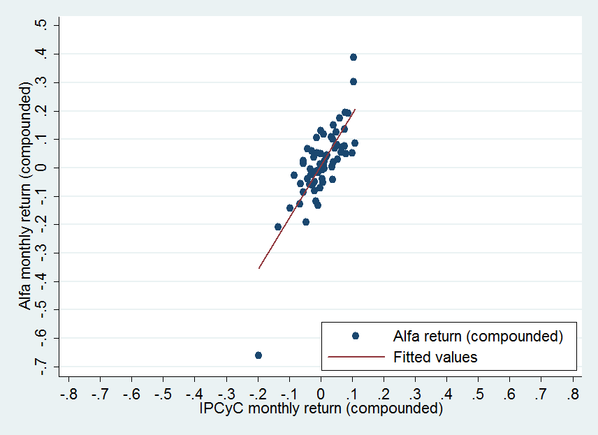
Then, if we take the company Alfa, S.A.B. de C.V. (one of these liquid firms), get its monthly stock prices from January 2007 to August 2012 and calculate the corresponding continuously compounded monthly returns, we can graphically examine how these returns are related with the continuously compounded market returns (those of the IPCyC). If we graph Alfa returns as the dependent variable in the Y axis, and the IPyC returns as the independent variable in the X axis, we would have:
A fitted line is shown in the graph. This fitted line pretends to represent the linear relationship between the monthly Alfa returns and the IPyC monthly returns. This line is the regression line, which represents the “conditional” mean of Y with respect to X.
We observe that for each increase in 10% of the IPyC return, the increase in the Alfa return is a bit higher than 10%. We can see this in the slope of the fitted line. For example, for 10% increase (0.1) of the IPyC return, the increase in the Alfa return is close to 15% or 17%. The slope of the fitted line represents the sensitivity of Alfa return with respect to changes in the market return. If the fitted line has a slope of 45 degrees, in other words, if it has a slope of 1, then on average for one percent increase in the IPyC, the percentage increase in the Alfa stock return will also be about one percent. If this line has a higher slope (closer to a vertical line), then the sensibility of Alfa with respect to the market will be very high.
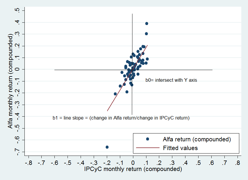
Mathematically we can express the expected return of Alfa as the conditional mean (that is the fitted line in the previous graph) as a simple linear relationship:
E(r_{alfa})=\hat{r}_{alfa}=b_{0}+b_{1}*r_{IPCyC}
In this case the dependent Y variable is the return of the stock Alfa (r_{alfa}), while the independent X variable is the return of the market (r_{IPCyC})
b_{0}=coefficient that represents where the fitted line crosses or intercept the Y axis. In this example, b_0 represents the expected monthly return of Alfa when the IPyC has zero monthly return.
b_{1}=coefficient that represents the slope of the line. This slope represents the average change of the dependent variable (Y) for one unit increase in the independent (X) variable. In this case, b_{1} represents the average change (in percentage points) in the monthly return of Alfa for +1% increase in the IPCyC.
Both b_{0} and b_{1} are called sample regression coefficients. We can see these regression coefficients graphically:
9.6 The Simple Regression Model
Besides estimating the expected value of the dependent variable Y using a linear relationship, we need to recognize that Y is a random variable, so we need to model this randomness or uncertainty adding a random shock or random error to the model. This stochastic model is the regression model and it is expressed as follows:
Y_i = \beta_0+\beta_1X_i+\varepsilon_i
Where \varepsilon_i is a random variable that follows a normal distribution:
\varepsilon_{i}\approx N(0,\sigma_{\varepsilon})
Thanks to the Central Limit Theorem then this error variable will behave like a Normal distributed variable since the error can be expressed as a linear combination of Y_i and X_i. The error term ε_t is expected to have mean=0 and a specific standard deviation σ_ε.
Unlike the regression line, the regression equation considers the stochastic error term \varepsilon_{i}, which represents each vertical distance from the regression line to each value of Y_i. Also, we add the subscripts i to indicate that the model applies to all specific sample values, from 1 to N -the number of observations.
If the error is positive, this means that the expected value falls short of the real Y_i value. If the error is negative, this means that the expected value overestimated the real Y_i value.
Considering the previous example for the expected value of Alfa return, we can express the corresponding regression model as:
r_{alfa_{t}}=b_{0}+b_{1}*r_{IPCyC_{t}}+\varepsilon_{t}
Where \varepsilon_{t} is a normal random error with mean zero and a specific standard deviation \sigma_{\varepsilon}. Then:
\varepsilon_{t}\approx N(0,\sigma_{\varepsilon})
In this example, each observation is one time period, so I used t subscript instead of i to indicate that each observation represents one time period. When we use a time-series dataset where each observation represents one time period and run a regression model, we call it a pulled-time-series regression model.
In the following section, we will review the types of regression models according to the type of data for the variables.
9.7 Types of data structures
The market model is a time-series regression model. In this model we looked at the relationship between 2 variables representing one feature or attribute (returns) of two “subjects” over time: a stock and a market index. The market model is an example of a regression model, but the data structure or type of data used is time-series data. These type of regression models are called pulled time-series regression.
There are basically three types of data used in regression models:
Time-series: each observation represents one period, and each column represents one or more variables, which are characteristics of one or more subjects. Then, we have one or more variables measured in several time periods. We call time-series regression model when the sample data is a time-series and the Y variable belongs to one subject. In the previous example, the subject was Alfa and the Y variable was its stock historical return.
Cross-sectional: each observation represents one subject in only one time period, and each column represents variables or characteristics of the many subjects.
Panel data: this is a combination of time-series with cross-sectional structure. This structure is also called long-format. When having this structure, it is recommended to use a panel-data regression model, which is similar to a multiple regression model, but it accounts for differences across subjects and time periods.
An example of a cross-sectional regression would be to analyze how annual earnings per share (when announced at the end of the year) of a set of 100 firms is related to the stock price change (return) of these firms right after the end of the year. In this case, the subjects are the 100 public firms; the dependent variable is the stock return of each of the 100 firms; and the independent variable would be the earnings per share of these 100 firms disclosed to investors at the end of the year. As we can see, we are looking only at one point in time, but we analyze the relationship between two variables or two features of the many subjects.
A panel-regression structure combines time-series with cross-sectional structures. Two different regression models can be run for a panel data structure. The first one is the pulled time-series regression. This regression model is the same as the time-series regression model but instead of having series of only one subject, we have series of more than one subject. The second regression model is called panel-data regression. Unlike the pulled time series model, this model accounts for changes in both subjects and periods. Taking the same example I gave for the cross-sectional regression, if we add 10 years of data for each of the 100 firms, then we would have a panel-data, so we can design either a) a pulled time-series regression, or b) a panel-data regression. For the pulled time-series regression, we run the regression as if all observations were from only one subject. For the panel-data regression model, we would need to estimate a more sophisticated model since there are basically two sources or types of relations: a) how changes in the dependent variable of subjects are related to changes in the independent variables of the same subjects, and b) how average (taking the average over time) changes in the dependent variable among different subjects are related to average changes in the independent variable. The first type of relation is called within-subjects differences, while the second one is called between-subjects differences. For now, we will not examine in detail panel-regression models, but it is important to have the distinction about the different types of regression models.
9.8 Assumptions of linear regression models
The main assumptions of the Linear Regresssion model are:
The model is linear in the sample regression coefficients
The errors of each observation are not correlated with the independent variable(s)
The mean of the errors is equal to zero.
The variance of the errors is constant for all observations
The errors are not correlated with each other
The number of observations must be greater than the number of coefficients to estimate (number of independent variables plus one)
The variance of the independent variables cannot be zero
9.9 Optimization methods to estimate regression coefficients
The most common methods to estimate regression coefficients are:
The Ordinary Least Squares (OLS) Method
Maximum Likelihood (ML)
The OLS method is the most common method for regression models. The OLS is simple and very fast to estimate. It tries to minimize the sum of all squared errors, which are the vertical distances from the real points to the regression line.
The ML method tries to maximize the probability (the likelihood) that predicted values from the model fit the real data points. ML is usually implemented with a numerical algorithm using loops to maximize the likelihood up to a threshold.
Next I will explain the OLS method
9.10 The OLS method
The simplest and most popular method to estimate the beta coefficients is the “Ordinary Least Square” (OLS) method.
The Ordinary Least Square is an optimization method to estimate the best values of the beta coefficients and their standard errors.
In the case of simple regression model, we need to estimate the best values of b_0 (the intercept) and b_1 coefficient (the slope of the regression line). If Y is the dependent variable and X the independent variable, the regression equation is as follows:
Y_i = b_0 + b_1(X_i) + \varepsilon_i
The regression line is given by the expected value of Y (also called \hat{Y}):
E[Y_i] = b_0 + b_1(X_i) = \hat{y}_i
In this case, i goes from 1 to N, the total number of observations of the sample.
If we plot all pairs of (x_i,y_i) we can first visualize whether there is a linear relationship between Y and X. In a scatter plot, each pair of (x_i,y_i) is one point in the plot.
The purpose of OLS is to find the best regression line that best represents all the points(x_i,y_i). The b_0 and b_1 coefficients define the regression line. If b_0 changes, the line moves up and down since its intercept moves. If b_1 changes, then the slope (inclination) of the line changes.
To find the best regression line (b_0 and b_1), the OLS method tries to minimize the sum of squared errors of the regression equation. Then OLS is an optimization method with the following objective:
Minimize \sum_{i=1}^{N}(y_{i}-\hat{y}_{i})^{2}
If we replace \hat{Y}_i by the regression equation we get:
This sum can be seen as a function of b_0 and b_1. If b_0 or b_1 change, this sum changes. Then we can re-write the optimization objective as:
Minimize:
f(b_{0},b_{1})=\sum_{i=1}^{N}\left[Y_{i}-(b_{0}+b_{1}X_{i}\right]^{2}
This is a quadratic function of 2 variables. If we get its 2 first partial derivatives (with respect to b_0 and b_1) and make them equal to zero we will get 2 equations and 2 unknowns - the beta coefficients- and the solution will be the optimal values of b_0 and b_1 that minimize this sum of squared errors. The set of these 2 partial derivatives is also called the gradient of the function.
If you remember basic geometry, if we imagine possible values of b_0 in the X axis and values of b_1 in the Y axis, then this function is actually a single-curved area (surface). The optimal point (b_0, b_1) will be the lowest point of this curved surface.
Let’s do an example with a dataset of only 4 observations:
X
Y
1
2
2
-1
7
10
8
7
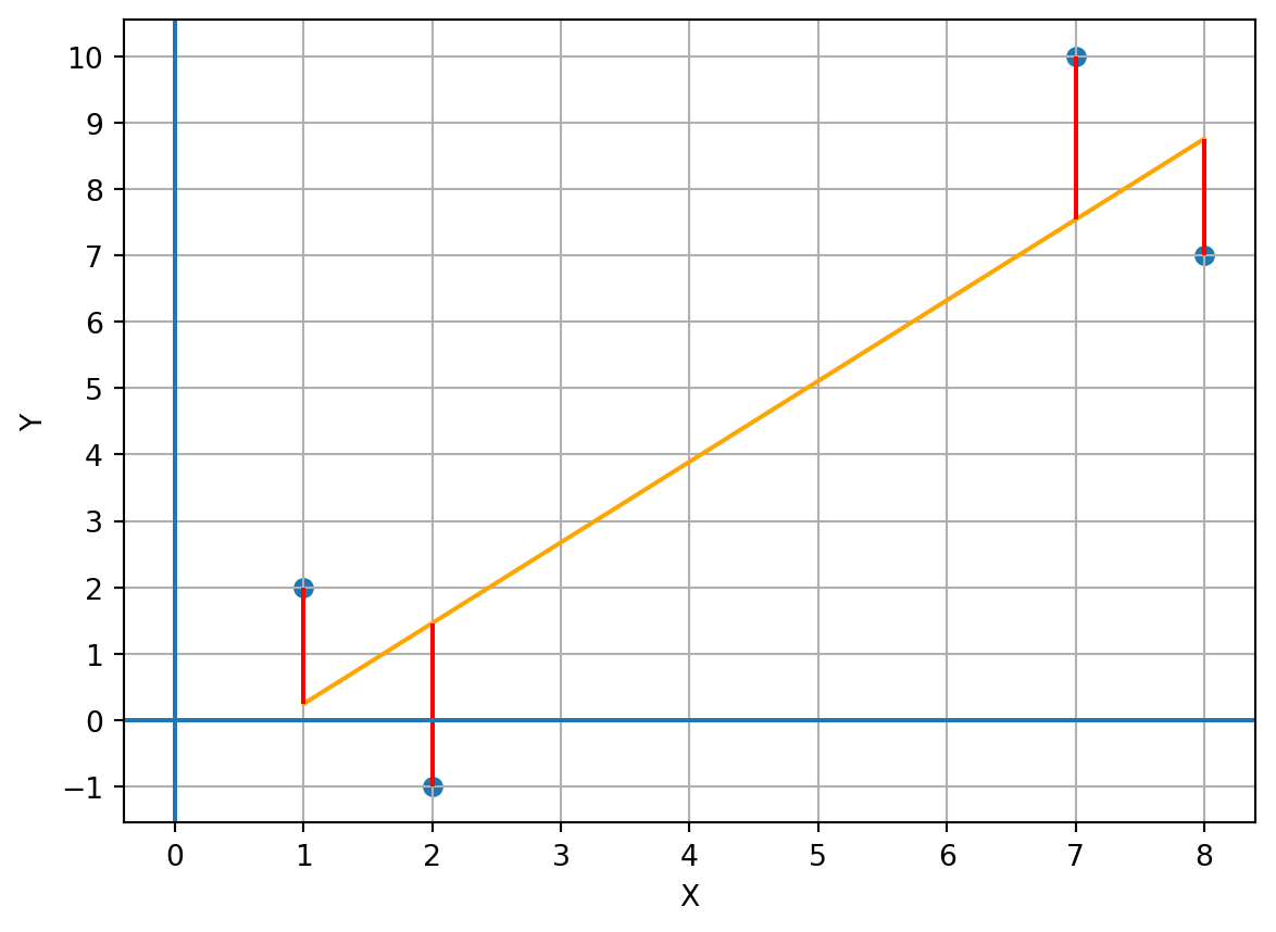
If I do a scatter plot and a line that fits the points:
Code
import pandas as pdimport matplotlibimport matplotlib.pyplot as pltimport numpy as np# I create a data frame with the X and Y columns and 4 observations to illustrate linear regression data = {'x': [1,2,7,8],'y': [2,-1,10,7]}df = pd.DataFrame(data)# I calculate the beta coefficients of the line equation that represents the points (the linear regression equation)b1,b0 = np.polyfit(df.x,df.y,1)# I calculate the regression equation with the coefficients:df['yhat'] = b0 + b1*df['x']#plt.clf()plt.scatter(df.x,df.y)plt.plot(df.x, df.yhat,c="orange")plt.xticks(np.arange(-4,14,1))plt.yticks(np.arange(-2,11,1))for i inrange(4): x=df.x.iloc[i] ymin= df.y.iloc[i] ymax=df.yhat.iloc[i]if (ymin>ymax): temp=ymax ymax=ymin ymin=temp plt.vlines(x=x,ymin=ymin,ymax=ymax,color='r')plt.axhline(y=0)plt.axvline(x=0)plt.xlabel("X")plt.ylabel("Y")plt.grid()plt.show()
The error of each point is the red vertical line, which is the distance between the point and the prediction of the regression line. This distance is given by the difference between the specific y_i value and its predicted value:
\varepsilon_i=(Y_i - \hat{Y}_i)
In this example, 2 errors are positive and 2 are negative.
The purpose of OLS is to find the values of b_0 and b_1 such that the sum of the squared of all errors is minimized. Why we square the errors? We square the errors as a trick to treat a negative error equal to a positive error. If we do not square the errors, then the sum can be very close to zero since the positive and the negative errors cancel each other out.
Mathematically there is only one solution to find the values of b_0 and b_1 that minimize the sum of squared errors.
Let’s return to the objective function, which is determined by both coefficients, b_0 and b_1.
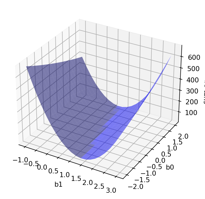
We can do a 3D plot for this function to have a better idea. It is a 3D plot since the function depends on 2 values: b_0 and b_1:
Code
from mpl_toolkits.mplot3d import Axes3Dimport matplotlib.pyplot as pltimport collections# I define a function to get the sum of squared errors given a specific b0 and b1 coefficients:def sumsqerrors2(b1, b0,df):returnsum( ( df.y - (b0+b1*df.x)) **2)# Note that df is a dataframe, so this line of code performs a row-wise operation to avoid # writing a loop to sum each squared error for each observation# Create the plot:fig = plt.figure()ax = fig.add_subplot(1,1,1, projection='3d')# I create 20 possible values of beta0 and beta1:# beta1 will move between -1 and 3b1s = np.linspace(-1, 3.0, 20)# beta0 will move between -2 and 2:b0s = np.linspace(-2, 2, 20)# I create a grid with all possible combinations of beta0 and beta1 using the meshgrid function:# M will be all the b1s values, and B the beta0 values:M, B = np.meshgrid(b1s, b0s)# I calculate the sum of squared errors with all possible pairs of beta0 and beta1 of the previous grid:zs = np.array([sumsqerrors2(mp, bp, df) for mp, bp inzip(np.ravel(M), np.ravel(B))])# I reshape the zs (squared errors) from a vector to a grid of the same size as M (20x20)Z = zs.reshape(M.shape)ax.plot_surface(M, B, Z, rstride=1, cstride=1, color='b', alpha=0.5)ax.set_xlabel('b1')ax.set_ylabel('b0')ax.set_zlabel('sum sq.errors')plt.show()
We see that this function is single-curved. The sum of squared errors changes with different paired values (b_0,b_1) considering the points (values of x_i and y_i) as fixed.
The lowest point of this surface will be the optimal values of (b_0, b_1) where the sum of squared error is the minimum of all. Then, how can we calculate this optimal point?
Remembering the basics of differential calculus and simultaneous equations, we can do the following:
Take the partial derivatives of the function with respect to its variables b_0 and b_1, and then make each partial derivative equal to zero to get 2 linear equations with 2 unknowns, and finally solve the linear equation:
Since \left[(y_{i}-(b_{0}+b_{1}*x_{i})\right] is the error for the i observation, then this Equation 9.1 states that the sum of all errors must be equal to zero.
Let’s do the same for the partial derivative with respect to b_1:
\sum_{i=1}^{N}(X_i)\left[Y_{i}-(b_{0}+b_{1}X_{i})\right]=0
\tag{9.2} Now we have 2 equations with 2 unknowns. I this case, the unknown variables are b_0 and b_1, since the X and Y values are considered as given or fixed.
We can now do simple algebra to solve for the values of b_0 and b_1. I will use the subtitution method to solve the system of equations.
We can further simplify both equations by applying the sum operator to each term:
\sum_{i=1}^{N}Y_{i}-N(b_{0})-b_{1}*\sum_{i=1}^{N}X_{i}=0
Since \bar{Y}=\frac{1}{N}\sum_{i=1}^NY_{i}, then \sum_{i=1}^{N}Y_{i}=N*\bar{Y}, and the same for the X variable, then:
N(\bar{Y})-N(b_0)-b1(N)(\bar{X})=0
Dividing both sides by N:
\bar{Y}-b_0-b_1(\bar{X})=0
This is another way to express Equation 9.1. This form of the equation indicates that the point(\bar{X},\bar{Y}) must be in the regression line since the error at this point is equal to zero!
From previous equation, then we get that:
b_0=\bar{Y} - b_1\bar{X}
After applying the sum to each term of Equation 9.2, it can be express as:
Interestingly, from this final formula for b_1, which is the slope of the regression line, we can see that b_1 is how much Y co-variates with X with respect to the variability of X. This is actually the concept of a slope of a line! it is the sensitivity of how much Y changes when X changes. Then, b_1 can be seen as the expected rate of change of Y with respect to X, which is a derivative.
How the b_1 coefficient and the correlation between X and Y are related? We learned that correlation measures the linear relationship between 2 variables. Also, b_1 measures the linear relationship between 2 variables, however, there is an important difference. Let’s see the correlation formula:
Corr(X,Y)=\frac{Cov(X,Y)}{SD(X)SD(Y)}
We can express Covariance in terms of Correlation:
Cov(X,Y)=Corr(X,Y)SD(X)SD(Y)
If we plug this formula in the b_1 formula:
b_1=Corr(X,Y)*\frac{SD(Y)}{SD(X)}
Then, we can see that b_1 is a type of scaled correlation since it is that is scaled by the ratio of both standard deviations, so b_1 provides information not only about relationship, but also about sensitivity of how much Y changes in magnitude for each change in 1 unit of X.
9.11 Regression statistics
The level of fitness of the regression model is measured with the coefficient of determination, also called R-squared. Before learning about the R-square, we need to learn about the three types of sum of squared deviations.
SST - Sum of squared deviations (Y_{i}-\bar{Y}). Each deviation represents the distance from each value of Y, Y_{i}, and its unconditional mean of Y. These deviations represent how each observation of the dependent variable Y is deviated from its unconditional mean. When I say unconditional mean I refer to the expected value of Y in the case X is omitted or is not considered as explanatory variable of Y. This unconditional mean is the arithmetic average of Y. Then the SST represents all deviations of Y from its average -its unconditional mean. The formula for the SST is:
SST=\sum_{i=1}^{N}(Y_{i}-\bar{Y})^{2}
SSRM - Sum of squared deviations of the regression model (\hat{Y}_{i}-\bar{Y}). Each deviation represents the distance from each conditional mean of Y and the unconditional mean of Y. The conditional mean is the expected value of Y given X (E[Y/X]) or the predicted value of Y using the fitted regression line. SSRM represents the squared deviations that are explained by the regression model. The formula for the SSRM is:
SSRM=\sum_{i=1}^{N}(\hat{Y}_{i}-\bar{Y})^{2}
Plugging the formula for \hat{Y}_i:
SSE - Sum of squared errors (Y_{i}-\hat{Y}_{i}). Each deviation represents the distance from each Y real value and its conditional mean or predicted Y value. the SSE represents how much of the total deviations of Y is not explained by the regression model. In other words, it represents the unexplained squared deviations of Y. The formula for SSE is:
SSE=\sum_{i=1}^{N}(Y_{i}-\hat{Y}_{i})^{2}
We can see that SST is composed of SSRM and SSE:
SST=SSRM+SSE
The total sum of squares of Y is equal to the explained sum of squares SSRM and the unexplained sum of squares SSE.
Now we introduce the R-squared statistic -also known as the coefficient of determination:
R^{2}=\frac{SSRM}{SST}
R^2 represents the proportion of the total Y variance that is explained by the corresponding regression model. We can also see that:
R^2=1-\frac{SSE}{SST}
If R^2=0.50 this means that the model explains 50% of the total Y variance.
An important statistic is the “variance” of the conditional mean Y, also called the variance of the model. This variance of the model equals to the variance of the regression errors.
According to the definition of variance of a variable, variance is the expected value of squared deviations of the variable from its mean - in this case, its conditional mean.
Then:
Var(Y/X)=E[Y-E[Y/X]]^{2}=E[Y-\hat{Y}]^{2}
We can compute this expected value as the average of the sum of squared errors(SSE), but we use N-2 as denominator instead of N. Then, this variance is computed as SSE divided by (N-2) since SSE is the sum of squared of errors:
Var(Y/X)=Var(\varepsilon)=\sigma_{\varepsilon}^{2}=\frac{SSE}{N-2}=MSE
The variance of the conditional Y is also called Mean Squared of Errors (MSE), and also is called the Variance of the Regression Errors. If we divide by N instead of N-2 we obtain a “biased” estimator of the true population variance of the conditional mean. We divide by N-2 to obtain an unbiased estimator since we have N-2 degrees of freedom because we have 2 parameters or coefficients to estimate: b_{0} and b_{1}.
Galton, Francis. 1886. “Family Likeness in Stature.”Proceedings of Royal Society 40: 42–72.
Gauss, Carl Friedrich. 1809. Theory of Motion of the Celestial Bodies Moving in Conic Sections Around the Sun.
Legendre, Adrien-Marie. 1805. Nouvelles Méthodes Pour La Détermination Des or-Bites Des Comètes.
Pearson, Karl Lee. 1930. The Life, Letters and Labors of Francis Galton.